FLORIDA B.E.S.T. · 2026–27
Algebra 1 EOC
Complete Study Guide
Understand the relationship. Choose a method. Check what your answer means. Build your Algebra 1 revision with detailed explanations, worked examples and original practice across the complete topic map.
37 chapters · 545 study topics · 6 original 48-question forms
PART 1 · CHAPTER 1
1. Introduction to Florida Algebra 1 EOC
Back to contents ↑1.1 What Is the Florida Algebra 1 EOC?
Florida’s Algebra 1 end-of-course assessment checks how well you reason with expressions, functions, data and equations after completing the course. Prepare to choose a model and interpret its result, not simply to remember a list of procedures. This guide follows the current B.E.S.T. course.
1.2 What Does B.E.S.T. Stand For?
B.E.S.T. means Benchmarks for Excellent Student Thinking. A benchmark describes a mathematical expectation; it is more specific than a chapter title. Use the benchmark map below to connect a skill, a worked explanation and an original diagnostic question.
1.3 Why Is the Algebra 1 EOC Important?
The result contributes to the course grade and is tied to Florida’s standard-diploma mathematics assessment requirement. These are separate decisions: earning course credit, meeting the assessment requirement and understanding the mathematics should each be checked with your school.
1.4 Who Must Take the Algebra 1 EOC?
Students enrolled in and completing the corresponding Algebra 1 courses participate, including Algebra 1, Honors and the listed equivalent courses. Retake, credit-acceleration and grade-forgiveness pathways have additional administration rules. Your school determines the correct registration and any individual provisions.
1.5 Middle School vs. High School Algebra 1 EOC
The course, rather than your age, determines the EOC. A middle-grades student enrolled in Algebra 1 takes its EOC instead of the grade-level mathematics assessment under the applicable statewide participation rule. The algebra expectations and score scale do not become easier for younger students.
1.6 Algebra 1 vs. Algebra 1 Honors EOC
Algebra 1 and Algebra 1 Honors use the same statewide Algebra 1 EOC. Honors teaching may include additional depth, pace or extension work. Prepare from the assessed benchmark inventory while continuing to complete the requirements of your own class.
1.7 Algebra 1 EOC vs. FAST Mathematics
FAST grade-level mathematics and the B.E.S.T. Algebra 1 EOC serve different courses and reporting purposes. Do not use a FAST grade-level score chart to interpret an Algebra 1 result. Practise the Algebra 1 sample interface and the course-specific mathematical content.
1.8 Algebra 1 EOC vs. Geometry EOC
Algebra 1 emphasizes relationships, equations and functions; Geometry emphasizes figures, transformations, measurement and geometric reasoning. Their current Level 3 thresholds differ. Algebra 1 is 400; Geometry is 404. Use the separate Geometry guide for that course rather than transferring its score bands here.
1.9 How Algebra 1 EOC Affects Your Final Course Grade
The statewide EOC component accounts for 30% of the final course grade under the applicable course-grade rule. A scale score is not already a percentage grade. Ask your school how it converts the EOC result and combines it with the remaining course work.
1.10 Algebra 1 EOC Graduation Requirements
For the usual Florida standard-diploma pathway, students must meet the Algebra 1 assessment requirement through the required passing result or an eligible comparative pathway. Cohort, transfer and disability provisions can affect an individual decision. Confirm your records with the school counselor; a local practice score cannot certify graduation eligibility. Students enrolled in the course must still participate in its EOC even when a passing comparative result is already on file.
1.11 What Students Should Know Before Preparing
Start with signed-number arithmetic, fractions, proportional reasoning and substitution. For example, evaluate before tackling a function table. If those foundations are slow, repair them alongside current algebra rather than spending every session on full mock tests.
1.12 How to Use This Review Guide
Attempt a diagnostic without the answer key, record the first decision you could not justify, then read that topic. Solve a fresh problem after the example and return after a gap. Use the chapter TOC, benchmark checkmarks and error log to choose your next session.
PART 1 · CHAPTER 2
2. Algebra 1 EOC 2027 Exam Format
Back to contents ↑2.1 Florida Algebra 1 EOC Exam Structure
The EOC is administered through the computer-based Test Delivery System. The current test is adaptive while maintaining its blueprint coverage. The original forms here are fixed study sets: they help you practise reasoning and response formats but do not reproduce the state’s selection or scoring system.
2.2 Number of Questions
The published blueprint gives approximately 45–50 items. Field-test items can be included, so do not assume the visible question count equals the number contributing to the reported score. Each original form on this page has exactly 48 items for a consistent study routine.
2.3 Exam Duration and Break Policy
The standard session is 160 minutes with a short break after 80 minutes. Students still working may continue up to the length of a typical school day under administration rules. Confirm your school’s arrangements and approved accommodations rather than treating the practice timer as an official time limit.
2.4 Computer-Adaptive Testing Explained
In adaptive testing, responses help determine later item difficulty, within content-coverage requirements. One difficult question does not reveal whether you are passing. Work from the mathematics in front of you; trying to infer your score from the order of easy and hard items is unreliable.
2.5 Multiple-Choice Questions
For a single-answer item, solve before comparing options when possible. In , the solution is 4; substitute it to confirm . Distractors may reflect a sign error, an unfinished step or a value for a different variable.
2.6 Multi-Select Questions
Read whether the instruction says select all or specifies a number of choices. Check each option independently against the condition. In this guide’s practice lab, a multi-select earns its one local point only when every required choice and no extra choice is selected.
2.7 Equation Editor Questions
An equation editor may require an expression, equation or numerical response. Keep parentheses around a complete numerator or denominator and check the displayed structure before moving on. For example, means something different from .
2.8 Graphing and Graphic Response Questions
A graph response can require a point, line or selected region. Read axis units and boundary rules first. To plot , use the intercept and another point such as , then verify both satisfy the equation.
2.9 Matching and Interactive Questions
Matching tasks require a complete set of correspondences, not a single plausible pair. Match a table to a function using at least two inputs and a structural feature such as a constant difference. Practise dragging or selecting in your school’s sample interface before test day.
2.10 Drop-Down and Hot-Text Questions
Drop-down and hot-text items ask you to complete a mathematical claim or select relevant information. Read the finished statement after every selection. A correct calculation can still produce an incorrect response if you select “decreasing” instead of “increasing” or confuse the initial value with the rate.
2.11 Calculator Availability and Rules
An online scientific calculator is available. A handheld must comply with current school and statewide policy; graphing, CAS, solver and regression features are prohibited. This page’s graphers and solvers are learning tools, not permission to use those functions during the EOC.
2.12 Official Formula and Reference Sheet
An official reference sheet is available in the test platform, with selected formulas and conversions. Learn how to locate and apply its entries before the exam. The larger OnlyPrepy formula sheet below is a revision resource and is not the official sheet supplied during testing.
2.13 Work Folders and Online Testing Tools
Use the supplied work folder for equations, sketches and checks. Label the question and define variables so you can revisit the reasoning. Practise the sample platform’s calculator, reference-sheet window, flagging and review controls; do not assume a home practice interface has identical behavior.
2.14 Testing Accommodations
Students with an eligible IEP or Section 504 Plan may receive specified accommodations, including accessible computer tools or approved paper formats when appropriate. Arrange these through school staff in advance. A study preference alone does not establish an accommodation, and this guide cannot determine eligibility.
2.15 How to Navigate the Computer-Based Test
Read directions, answer in the required format, flag uncertain items when the platform permits it and review before submitting. Check that a graph point or selection actually registered. If equipment fails, notify the proctor immediately instead of opening another application or attempting your own repair.
PART 1 · CHAPTER 3
3. Algebra 1 EOC Scores, Passing & Retakes
Back to contents ↑3.1 Algebra 1 EOC Score Scale Explained
Current B.E.S.T. Algebra 1 results use a scale from 325 to 475. A scale score summarizes performance through the state’s scoring model. It is not the number correct, a percentage out of 100 or the score scale used by every other Florida assessment.
3.2 Achievement Levels 1–5
The current Algebra 1 bands are Level –378; Level –399; Level –417; Level –434; and Level –475. Level 3 represents on-grade-level performance. Interpret an actual report using the score tool below.
3.3 What Is a Passing Algebra 1 EOC Score?
The current B.E.S.T. Algebra 1 Level 3 threshold is 400. A score of 399 remains in Level 2; 400 enters Level 3. Historical tests and individual alternative provisions should be reviewed separately rather than mixed into this current achievement-band table.
3.4 Minimum Passing Score for Graduation
For the usual current assessment pathway, 400 meets the B.E.S.T. Algebra 1 passing threshold. Whether a student has satisfied the complete graduation requirement also depends on the applicable records and provisions. Ask the counselor to confirm the requirement as met in the student record. The published alternate passing score is 398 for eligible earlier B.E.S.T./FSA pathways; it is not the current Level 3 boundary. Eligibility depends on the first administration and applicable assessment requirement.
3.5 How the 30% Course-Grade Rule Works
Suppose a school converts an EOC result to 80 on its grading system and the other course component is 90. A combination gives . The 80 is a hypothetical converted grade, not a formula for converting the state scale score.
3.6 How Computer-Adaptive Scoring Works
Adaptive scoring considers the calibrated items and response pattern through the state’s model. Two practice attempts with the same percentage do not establish equal official scores. The useful study question is which concepts remain unreliable, not which invented raw-score conversion looks most reassuring.
3.7 Raw Score vs. Scale Score
A raw score counts earned item credit under a test’s rules; a scale score places performance on an established reporting scale. This page reports one local point per original practice item. It has neither the state’s calibration nor a valid raw-to-scale conversion.
3.8 Why There Is No Universal Passing Percentage
There is no universal percentage that guarantees 400. Item difficulty, scoring and the adaptive assessment design prevent a simple public rule such as “60% always passes.” Track practice accuracy across fresh comparable sets, but describe it as practice evidence rather than a passing prediction.
3.9 Understanding Your EOC Score Report
Read the test name, administration date, scale score, achievement level and reporting-category information together. Compare category evidence with your actual work before deciding what to revise. Ask the school for access to the report if your family portal is not yet showing it.
3.10 What Happens If You Fail the Algebra 1 EOC?
A non-passing result means the assessment requirement needs further attention; it does not by itself explain every course-credit or graduation outcome. Meet the counselor, identify the available retake or eligible alternative pathway, and bring a specific plan for repairing recurring mathematical weaknesses.
3.11 Retaking the Algebra 1 EOC
Retakes occur in scheduled administration windows through the school. Ask about the next available window, registration and any required instruction. Between attempts, work from category evidence and fresh questions; repeatedly memorizing one practice form can hide the weakness you need to address.
3.12 Alternative Comparative Scores and Eligibility
For students who entered Grade 9 in 2020–21 or later, the current comparative table includes SAT Math 420; PSAT/NMSQT or PSAT 10 Math 430; ACT or PreACT Secure Math 16; CLT or CLT10 Quantitative Reasoning 14; or Geometry EOC Level 3. Historical cohort and test-date provisions can differ. Have the counselor verify eligibility and the recorded result using the September 2026 requirements document.
3.13 Algebra 1 EOC Score Estimator and Limitations
The tool here interprets an actual reported score only. Practice results show local accuracy and missed skills. Neither is an official forecast, a guarantee of passing nor a substitute for your school’s graduation review. No score or attempt is sent to a state testing system.
3.14 How to Improve Your Performance
For every missed item, identify whether the issue was translation, method, arithmetic, response entry or interpretation. Correct the first wrong step, solve a new version unaided and revisit it several days later. A steadily shorter list of recurring errors is more actionable than a single higher percentage.
Current Algebra 1 achievement bands
| Level | Scale-score band | Interpretation |
|---|---|---|
| 1 | 325–378 | Below the current Level 3 threshold |
| 2 | 379–399 | Below the current Level 3 threshold |
| 3 | 400–417 | On grade level; current passing threshold starts at 400 |
| 4 | 418–434 | Above Level 3 |
| 5 | 435–475 | Highest achievement band |
These are current achievement bands. Historical alternate passing eligibility is a separate school-record decision.
Interpret your reported score →PART 1 · CHAPTER 4
4. Florida B.E.S.T. Algebra 1 Standards & Blueprint
Back to contents ↑4.1 Overview of the Official B.E.S.T. Mathematics Standards
The standards describe the course, while the assessment blueprint identifies the benchmark inventory and reporting balance for this test. Some course activities are foundations or extensions. Keep both in view: meet classroom expectations and prepare deliberately for the assessed relationships.
4.2 Reporting Category 1: Expressions, Functions, and Data Analysis
Expressions, Functions, and Data Analysis covers number reasoning, equivalent expressions, function interpretation and data displays. It represents 31–38% in the published blueprint. Practise switching between equations, tables, graphs and verbal descriptions rather than treating each representation as an unrelated topic.
4.3 Reporting Category 2: Linear Relationships
Linear Relationships includes equations, inequalities, lines, systems and linear data models. Its published share is 31–38%. Show how a solution meets every constraint, explain a slope in units and distinguish an algebraic result from a viable answer in context.
4.4 Reporting Category 3: Non-Linear Relationships
Non-Linear Relationships includes polynomial work, quadratics, absolute value, exponentials and financial models. It also has a 31–38% share. Compare the operation driving change: constant additions suggest a line; constant multiplication suggests an exponential relationship.
4.5 Complete Assessed Benchmark List
The map below lists all 46 entries in the published Algebra 1 inventory: 43 primary benchmark entries and three supporting “also assesses” entries. Supporting entries remain worth studying. Each row connects to a chapter and an original diagnostic task; these study connections are not official item assignments.
4.6 Understanding Benchmark Codes (MA.912...)
In MA.912.AR.2.1, MA identifies mathematics, 912 identifies the high-school grade band and AR identifies algebraic reasoning. The remaining numbers locate the standard and benchmark. Use the complete code in your error log so similarly named skills are not confused.
4.7 Mathematical Thinking and Reasoning Standards
Mathematical Thinking and Reasoning expectations run through the content: make sense of a problem, represent a relationship, justify a step, recognize structure and check whether a result is reasonable. A correct option without a defensible method is weak preparation for a changed problem.
4.8 Conceptual Understanding vs. Procedural Fluency
Procedural fluency is carrying out a method accurately; conceptual understanding is knowing why it fits. Solve by division, then explain that division by 3 preserves equality. Practise both so a slightly unfamiliar presentation does not stop you.
4.9 Real-World Mathematical Modeling
Modeling starts with quantities and assumptions. If a taxi costs USD 4 plus USD 2 per mile, define as miles and write for . Interpret the 4 and 2 with units, then check whether the model’s assumptions fit the question.
4.10 Identifying Important Exam Topics
All three reporting categories have substantial weight, so skipping statistics or exponentials is risky preparation. Prioritize high-frequency personal errors within the full benchmark map. A long revision list becomes manageable when each session ends with a small set of skills you can now explain unaided.
4.11 Cognitive Difficulty and Multi-Step Reasoning
A multi-step task may combine a function model, equation solution and contextual restriction. Pause at each transition: what quantity do I need, which relationship connects it, and what conditions make the result valid? Increasing difficulty does not always mean longer arithmetic.
4.12 Standards-to-Chapters Alignment Table
Use the study-connection column in the benchmark table to locate the relevant chapter. For instance, function features lead to Chapters 7–8 and quadratics to Chapters 20–21. The table is a navigation aid; the chapter notes explain the actual mathematical conditions.
4.13 Benchmark-to-Practice-Question Coverage Tracker
Mark a benchmark reviewed after reading its explanation and attempting its linked diagnostic question. Browser checkmarks record review, not certified mastery. A stronger personal standard is two successful fresh attempts, separated in time, with a written explanation of the critical step.
All 46 blueprint entries: study and original-practice connections
The 43 primary entries and three supporting “also assesses” entries below follow the published blueprint inventory. Chapter and question links are OnlyPrepy study connections. “Reviewed” records your review on this browser; it is not a mastery certification.
0 of 46 benchmark entries reviewed
PART 2 · CHAPTER 5
5. Algebra Fundamentals & Expressions
Back to contents ↑5.1 Introduction to Algebraic Expressions
An expression names a quantity without asserting equality. In , the value changes with ; an equation such as imposes a condition. Decide whether the question asks you to simplify, evaluate, solve or interpret before choosing an operation.
5.2 Variables, Constants, Terms and Coefficients
In , the terms are , and ; coefficients are and 5, is constant. The minus sign belongs to its term. Keeping signs attached prevents errors when rearranging or combining expressions.
5.3 Order of Operations (PEMDAS)
Evaluate grouping first, then exponents, then multiplication/division left to right, then addition/subtraction left to right. Thus , not 3. A fraction bar groups the entire numerator and denominator even when ordinary parentheses are not printed.
5.4 Properties of Real Numbers
Real-number properties justify equivalent steps. Adding zero changes nothing, multiplying by one changes nothing and a nonzero number times its reciprocal equals one. Division by zero is undefined; canceling a variable requires considering whether that variable could be zero.
5.5 Commutative, Associative and Distributive Properties
Commutative changes order, associative changes grouping and distributive multiplies every term inside a sum. For example, . Subtraction and division are not commutative: and have different values.
5.6 Translating Words into Algebraic Expressions
“Five less than twice a number” becomes ; “five minus twice a number” becomes . Define the variable and translate the relationship in its original order. Test a small number to see whether your expression matches the words.
5.7 Evaluating Algebraic Expressions
Substitute each value with parentheses before calculating. For at , write . Squaring a negative input and placing a negative sign outside a square are different operations.
5.8 Combining Like Terms
Like terms have identical variable parts and exponents. Combine to get , but do not combine and . You add coefficients, retaining the shared variable part rather than adding its exponent.
5.9 Simplifying Multi-Step Expressions
Distribute first, collect like terms and keep each sign visible. For , expand to . A quick substitution at confirms both versions give , although one check alone does not prove general equivalence.
5.10 Equivalent Expressions
Equivalent expressions agree for every allowed input. Factoring into preserves the value by distributivity. Numerical spot checks can disprove equivalence, but a symbolic property is the stronger way to establish that two expressions always agree.
5.11 Identifying Parts of Equations and Formulas
An equation has two expressions joined by equality. In , depends on base and perpendicular height. Identify what each symbol measures and any restrictions before rearranging; a formula should retain consistent units on both sides.
5.12 Rearranging and Solving Literal Equations
To isolate in , multiply by 2 and divide by : , assuming . Apply the same operation to both sides. State restrictions when a step divides by a quantity that may be zero.
5.13 Real-World Algebraic Modeling
A subscription with a USD 12 setup charge and USD 8 per month is . The setup fee is paid once, not multiplied by months. If the question allows only complete months, the practical domain is nonnegative integers rather than all real numbers.
5.14 Common Mistakes in Algebraic Expressions
Watch for losing a negative sign, combining unlike terms and reversing subtraction in a translation. Write one operation per line and compare structure before calculating. If a simplified expression has an unexpected degree or changes the value at an easy input, revisit the first transformation.
PART 2 · CHAPTER 6
6. Exponents, Radicals & Number Systems
Back to contents ↑6.1 Understanding Real Numbers
Real numbers include rational and irrational numbers on the number line. Integers and terminating or repeating decimals are rational; is irrational. In Algebra 1, check real-number restrictions when taking an even root or dividing by an expression.
6.2 Rational vs. Irrational Numbers
A rational number can be written as a ratio of integers with nonzero denominator. A nonterminating decimal is not automatically irrational: . Nonterminating, nonrepeating decimals are irrational. A calculator’s rounded display cannot establish rationality by itself.
6.3 Integer and Rational Exponents
An integer exponent counts repeated multiplication when positive. Rational exponents connect powers with roots: . Over the real numbers, an even denominator in a reduced exponent requires suitable nonnegative bases.
6.4 Product of Powers Rule
For a common base, multiplication adds exponents: . This rule does not say . Read the operation between terms before selecting an exponent law.
6.5 Quotient of Powers Rule
For a nonzero common base, division subtracts exponents: . Keep the nonzero restriction. If the exponent difference is negative, rewrite with a positive exponent in the denominator rather than making the value negative.
6.6 Power of a Power Rule
A power raised to a power multiplies exponents: . A power of a product acts on every factor: . Compare this with , where only is cubed.
6.7 Zero and Negative Exponents
For , and . A negative exponent indicates a reciprocal, not a negative number. Thus , while .
6.8 Fractional Exponents and Radicals
Use where defined. For example, . The principal square root is nonnegative: . Solving is a different task and gives both 5 .
6.9 Simplifying Exponential Expressions
Simplify for nonzero . The numerator is , giving . Record restrictions from the original expression even if a variable disappears during simplification.
6.10 Simplifying Square Roots
Extract perfect-square factors: . For variables, over all real . Replacing the absolute value with requires a nonnegative-variable assumption.
6.11 Adding and Subtracting Radical Expressions
Combine radicals only after simplifying their radicands. . In general, is not .
6.12 Multiplying and Dividing Radical Expressions
For nonnegative radicands, . Thus . For division, the denominator must be positive in ; rationalizing a denominator is an equivalent rewrite, not a change of value. For cube roots, negative radicands are also real: the cube root of times the cube root of 27 equals .
6.13 Converting Between Radical and Exponential Forms
In , the reduced denominator indicates the root and the numerator indicates the power. For positive , . State a real-number domain when rewriting expressions involving even roots.
6.14 Estimating and Comparing Expressions
Bound irrational values between known squares. Since , . When comparing positive expressions, squaring can preserve order; squaring signed numbers without checking signs can reverse the apparent comparison.
6.15 Multi-Step EOC Exponent and Radical Problems
Evaluate : first simplify to . Separate exponent rules from radical rules, keep exact values during working and round only if the question requests a decimal.
PART 2 · CHAPTER 7
7. Introduction to Functions
Back to contents ↑7.1 What Is a Function?
A function assigns exactly one output to each input in its domain. Different inputs may share an output. The function gives the same output for 2 without violating the definition.
7.2 Relations vs. Functions
A relation is any set of input-output pairs; a function is a relation with no input assigned two different outputs. The pairs fail the function rule. Repeated outputs such as are allowed.
7.3 Domain and Range
The domain contains permitted inputs and the range contains produced outputs. For , the real domain and range are both nonnegative. In a story, additional restrictions may apply: ticket counts must be whole numbers even if the formula accepts fractional inputs.
7.4 Independent and Dependent Variables
The independent variable is the chosen input; the dependent variable responds to it. If total cost depends on the number of tickets, ticket count is independent and cost dependent. Assign units to both before interpreting slope or drawing axes.
7.5 Function Notation: f(x)
The notation means the value of function at input , not multiplication of by . In , . The function name can change without changing this input-output idea.
7.6 Evaluating Functions
Replace every occurrence of the input with the given value. For , . Using parentheses prevents a sign error when the input is negative.
7.7 Functions from Tables
Check a table for repeated inputs with conflicting outputs. Then inspect equal input intervals for a pattern. A constant output difference across equal input steps suggests a linear model; unequal input steps require comparing rates rather than raw differences.
7.8 Functions from Graphs
The vertical-line test checks whether a graph assigns more than one output to an input. A circle fails because some vertical lines meet it twice. Read filled and open endpoints carefully when stating the domain and range of a restricted graph.
7.9 Functions from Equations
An equation may define a function when it supplies one output per allowed input. does; does not define as a single-valued function of positive unless a branch is specified.
7.10 Functions from Verbal Descriptions
“A tank begins with 50 liters and loses 3 liters each minute” gives while the tank contains water. The meaningful time domain ends when the tank empties. The algebraic line continues beyond that interval, but the physical model does not.
7.11 Identifying Linear, Quadratic, Absolute Value and Exponential Functions
Recognize line, parabola, V-shape and repeated-factor growth. Typical models are , , and . A finite table can fit multiple functions, so use stated assumptions and structural evidence rather than claiming certainty from a few values.
7.12 Comparing Functions in Different Representations
Compare like features: intercept with intercept, average rate over the same interval with average rate, and outputs at the same input. A table’s first row is not necessarily the initial value unless its input is zero.
7.13 Interpreting Functions in Real-World Contexts
In , 120 is the initial population in the model and 1.04 is the annual factor if counts years. Do not describe 1.04 as a 104% increase; the increase is 4% per stated period.
7.14 Function Evaluation Practice
Try : find , and the inputs producing 7. The first two are and 7; solving gives . Evaluating an output and solving for an input are different operations.
PART 2 · CHAPTER 8
8. Graphs, Function Features & Transformations
Back to contents ↑8.1 Cartesian Coordinate Plane
The horizontal coordinate is written first in . Quadrants organize sign pairs: , , and . Check the scale on each axis; equal visual spacing need not represent equal numerical increments across different graphs.
8.2 Intercepts and Zeros
A y-intercept occurs where ; an x-intercept or zero occurs where . For , these are and . State whether the question asks for a coordinate point or just the zero’s x-value.
8.3 Intervals of Increase and Decrease
Read a graph from left to right. A function increases when outputs rise as inputs increase, and decreases when outputs fall. For , it decreases on and increases on .
8.4 Maximum and Minimum Values
A maximum is the greatest output in the specified domain; a minimum is the least. The parabola has maximum value 4 at input 1. Distinguish the extremum value from the point .
8.5 Positive and Negative Function Intervals
Positive-function intervals are where the graph lies above the x-axis, not where the graph is increasing. For , outputs are positive when or and negative between the zeros.
8.6 Average Rate of Change
Average rate of change is for distinct inputs. For from 1 to 3, it is . It describes the secant-line rate across an interval, not a constant rate everywhere.
8.7 Recognizing Linear vs. Nonlinear Graphs
A linear function has constant rate of change and a straight graph. A curve, V-shape or a changing rate indicates a nonlinear function. A nearly straight short section of a curve does not prove that the entire relationship is linear.
8.8 Parent Functions
Useful parent functions are , , and for , . Know their basic shapes, intercepts and ranges before adding transformations. Transformations are easier to interpret when you can identify the starting structure.
8.9 Vertical and Horizontal Translations
Adding outside moves vertically: shifts up . Replacing the input with shifts right . Thus has its vertex at ; the inside sign often causes the first mistake.
8.10 Reflections of Functions
A negative multiplier outside reflects across the x-axis: . Replacing the input with reflects across the y-axis: . Even functions such as already have y-axis symmetry, so their reflected graph may look unchanged.
8.11 Vertical Stretches and Compressions
Multiplying outputs by stretches vertically when and compresses when ; a negative also reflects. Compare and at the same input to see the change directly.
8.12 Interpreting Transformed Functions
For , identify the right shift of 1, vertical stretch by 2, x-axis reflection and upward shift of 3. The vertex is and the range is . Describe each change relative to the parent. Replacing by compresses horizontally by a factor of ; stretches horizontally by 2. The input multiplier acts reciprocally on horizontal coordinates.
8.13 Comparing Function Features from Graphs, Tables and Equations
A graph can show a vertex, a table can bracket it and an equation can locate it exactly. Compare features at a common level of precision. Sparse table values alone may not reveal the exact turning point without an assumed function model.
8.14 Real-World Graph Interpretation
A distance-time graph’s slope represents speed only when the plotted quantity and context support that interpretation. A horizontal segment means the plotted distance stays constant. A downward segment can mean movement back toward a reference point, not negative elapsed time.
PART 2 · CHAPTER 9
9. Descriptive Statistics & Data Displays
Back to contents ↑9.1 Types of Statistical Data
Statistical data describe cases and variables. Record who or what was measured, the measurement units and how the sample was obtained. A neatly computed mean can still mislead if the sample excludes much of the population you want to discuss.
9.2 Categorical vs. Numerical Data
Categorical data classify, such as transport type; numerical data measure or count, such as travel minutes. A number used as a label, like a jersey number, is categorical. Choose graphs and summaries that match the actual variable rather than its appearance.
9.3 Univariate vs. Bivariate Data
Univariate data study one variable; bivariate data pair two measurements for each case. A scatter plot of study hours and scores must preserve the student-by-student pairs. Two separate lists without their original pairing cannot support the same association analysis.
9.4 Mean, Median, Mode and Range — Foundation Review
For , mean is 4, median is 3, mode is 3 and range is 6. Sort before finding the median. The range measures spread, not a typical value, and the mode may be absent or nonunique.
9.5 Measures of Center and Spread
Pair a center with a suitable spread. Mean and standard deviation describe many roughly symmetric distributions; median and interquartile range resist extreme values better. State what the chosen statistics reveal about typical size and variability rather than reporting unexplained numbers.
9.6 Dot Plots and Histograms
A dot plot keeps individual values visible; a histogram groups numerical values into intervals. Histogram bar heights depend on interval definitions. Do not read a histogram as if each bar were a named category or assume you can recover every original measurement.
9.7 Box-and-Whisker Plots
A box plot summarizes minimum, lower quartile, median, upper quartile and maximum, with outlier conventions sometimes modifying whiskers. A longer box indicates a larger interquartile range. The length of a section does not mean it contains more observations than another quartile section.
9.8 Quartiles and Interquartile Range
The interquartile range is and describes the middle half of the data. For and , IQR is 8. Quartile conventions can differ in small samples; follow the method or provided quartiles in the question.
9.9 Identifying Outliers
A common outlier rule flags values below or above . With quartiles 12 and 20, the fences are 0 and 32. A flagged value deserves investigation; it is not automatically an error to delete.
9.10 Interpreting Data Distributions
Describe shape, center, spread and unusual values together. A right-skewed distribution has a longer tail toward larger values, often pulling the mean above the median. The tallest bar alone does not describe the complete distribution.
9.11 Comparing Data Sets
Compare the same statistic and units for both groups. If medians are 20 and 24 minutes but IQRs are 4 and 12, the second group has a higher middle value and greater middle-half variability. Avoid claiming every value in the second group is larger.
9.12 Two-Way Frequency Tables
A two-way frequency table cross-classifies cases by two categorical variables. Interior cells give joint counts, row and column totals are marginal counts, and the grand total counts all cases once. Verify totals before computing percentages.
9.13 Joint, Marginal and Conditional Relative Frequencies
Joint relative frequency divides a cell by the grand total; conditional relative frequency divides by the relevant row or column total. If 12 of 20 bus riders are early among 50 students, joint frequency is while early-given-bus is .
9.14 Recognizing Associations in Categorical Data
Compare conditional percentages across groups to investigate association. If 60% of one group and 30% of another report the same outcome, the sample suggests an association. Different group sizes make comparing raw counts alone unreliable, and association does not establish causation.
9.15 Choosing Appropriate Data Representations
Use a histogram or box plot for a numerical distribution, a bar chart for categorical counts, a scatter plot for paired numerical variables and a two-way table for paired categories. Match the representation to the question you want to answer.
9.16 Data Analysis Word Problems
In a survey, 18 of 30 cyclists and 20 of 50 drivers arrive before 8. The early-arrival rates are 60% and 40%, respectively. Although more drivers arrive early in count, cyclists have the higher conditional rate. Name the denominator in your explanation.
PART 2 · CHAPTER 10
10. Comparing Functions & Applied Data Analysis
Back to contents ↑10.1 Comparing Linear, Quadratic and Exponential Functions
Across equal input steps, linear outputs have constant first differences, quadratics have constant second differences, and exponentials have constant ratios when defined. Use these patterns with the model assumptions. A finite number of values does not uniquely determine an arbitrary function.
10.2 Comparing Initial Values
Compare initial values at input zero. For and , the initial values are 40 and 30. A larger initial value does not guarantee a larger value at every later time.
10.3 Comparing Rates of Change
A line’s rate is constant; nonlinear average rates depend on the interval. Compare both functions over the same input interval with the same units. A 5-unit increase per year cannot be compared directly with a 5% annual increase without considering the current quantity.
10.4 Constant Differences vs. Constant Ratios
The sequence adds 3 each step; multiplies by 2. The first is linear in the index and the second exponential. Divide consecutive nonzero outputs when checking a ratio, and subtract when checking a difference.
10.5 Average Rate of Change from Tables
From a table with and , average rate is . Divide by the actual input change, not by the number of table rows. Intermediate values are unnecessary for this interval’s average rate.
10.6 Average Rate of Change from Graphs
Read two plotted coordinates carefully, then use change in output over change in input. If a graph rises from to , the average rate is output units per input unit. Check that the axis intervals were read correctly.
10.7 Function Growth and Long-Term Behavior
For a growth factor greater than 1, an exponential eventually exceeds a positive linear or polynomial growth model as input increases without bound. That does not tell you which is larger over a short practical interval. Compare actual values within the stated domain.
10.8 Determining the Best Function Model
Use context, pattern and residual evidence together. Constant-dollar growth suggests a line; repeated-percentage change suggests an exponential. A parabola may fit a rise-and-fall process. A model fitting given points is not automatically a trustworthy forecast outside the observed range.
10.9 Interpreting Function Parameters
In , 25 is the fixed starting cost and 4 is the cost per unit. In , 200 is initial value and 0.8 retains 80% each period. Explain parameters in the model’s units and time scale.
10.10 Financial and Scientific Modeling Examples
A savings balance without extra deposits can follow a compound-growth model; a tank draining at a constant volume per minute follows a line. Define assumptions such as a constant rate and no added withdrawals. A correct formula applied to the wrong process is still a poor model.
10.11 Multi-Representation Comparison Questions
Suppose a table gives and . The first function’s average rate over 0–2 is 3; the second’s is 4. Their starting values are 8 and 1. Compare the requested feature instead of choosing one function as universally “greater.”
10.12 Mixed Reporting Category 1 Practice Test
Use the practice lab’s Category 1 topic choices for expressions, exponents, functions and data, or attempt Questions 1–16 of a fixed form. Review each wrong answer’s benchmark and chapter before moving on. Local item counts are balanced study design, not a replica of adaptive test scoring.
PART 3 · CHAPTER 11
11. Solving Linear Equations
Back to contents ↑11.1 What Is a Linear Equation?
A one-variable linear equation can be reduced to , with , by equivalent operations. The variable is not squared or placed in an exponent. An equation like is a contradiction, not an ordinary unique-solution linear equation.
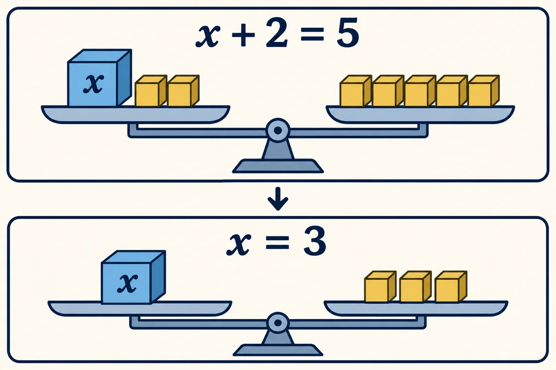
11.2 One-Step Linear Equations
Undo the operation applied to the variable. For , add 7 to both sides to get 19. For , divide both sides to get . Substitute the value into the original equation to check.
11.3 Two-Step Linear Equations
For , subtract 5 first, giving , then divide by 3 to obtain . Reverse the order of the operations on the unknown. Keep both sides balanced rather than “moving” terms without tracking their signs.
11.4 Multi-Step Linear Equations
Expand brackets, combine like terms and isolate the variable. In , simplify to , then and . Writing intermediate lines exposes the step to revisit if substitution fails.
11.5 Equations with Variables on Both Sides
For , subtract and add 4 to obtain , so . You can collect variables on either side; choose the side that keeps arithmetic clear. Do not subtract a term from only one side.
11.6 Equations with Fractions and Decimals
Clear denominators using a common multiple applied to every term. For , multiply the whole equation by 6: , giving . With decimals, preserve place value and check the unrounded original equation.
11.7 Using the Distributive Property
For , distribute to or divide both sides first. Either valid route gives . A negative outside parentheses acts on each term, including a negative constant.
11.8 Equations with No Solution
If variable terms cancel and leave a false statement, there is no solution. For , subtracting gives . No value of can repair that contradiction.
11.9 Equations with Infinitely Many Solutions
If simplification leaves a true statement such as , every allowed input is a solution. For , both sides are identical. Say “all real numbers” when no original restrictions exclude any values.
11.10 Solving Literal Equations
In , solve for by dividing by : . When isolating a variable appearing more than once, collect and factor it first. State any nonzero assumptions introduced by division.
11.11 Writing Equations from Word Problems
If a gym charges USD 15 to join and USD 9 per visit, a total of USD 60 means . Subtract 15 and divide by 9 to obtain 5 visits. Define before writing the equation and keep cost and count units distinct.
11.12 Interpreting Solutions in Real-World Contexts
A calculated ticket count of 4.5 may be algebraically valid but impossible if tickets are indivisible. Apply domain and situation restrictions after solving. Sometimes this means there is no feasible exact answer; do not round silently unless the question asks for a minimum or maximum whole number.
11.13 Checking and Verifying Solutions
Substitute a candidate into both sides of the original equation. For and , both sides equal 13. Checking only the last simplified line may miss an earlier invalid operation or restriction.
11.14 Common Algebra 1 EOC Equation Mistakes
Common errors include distributing to only one term, changing a sign incorrectly and dividing only part of a side. Annotate the operation beside each line. If a solution fails the original equation, compare consecutive lines to locate the first loss of equivalence.
PART 3 · CHAPTER 12
12. Linear Inequalities
Back to contents ↑12.1 Introduction to Linear Inequalities
An inequality describes an ordered comparison and usually a set of solutions. For , subtract 2 to obtain . Values such as 4 work, while the boundary value 5 does not because the comparison is strict.
12.2 Inequality Symbols and Number Lines
Use an open endpoint for or and a closed endpoint for or . Shade toward smaller numbers for and toward larger numbers for . The endpoint style communicates whether the boundary itself is included.
12.3 Solving One-Step Inequalities
Add or subtract the same number on both sides without reversing the symbol. From , get . If dividing by a positive number, retain the direction; becomes .
12.4 Solving Multi-Step Inequalities
Distribute and collect terms as for equations, watching the sign of the final divisor. For , simplify to , then . Test a value on each side of the boundary to check the set.
12.5 Multiplying and Dividing by Negative Numbers
Multiplying or dividing both sides by a negative reverses the comparison. From , divide to obtain . The number line explains why: multiplication by a negative reverses order.
12.6 Compound Inequalities
“And” means intersection; “or” means union. The compound statement requires both conditions. The set or has two separate rays. Do not join the rays through the excluded middle interval.
12.7 Graphing Inequalities on Number Lines
Solve algebraically before graphing, then mark the boundary and direction. For , place a closed point and shade right. A test value such as 0 confirms the chosen direction.
12.8 Writing Inequalities from Real-World Situations
“At most USD 50” means a cost no greater than 50. With a USD 10 fee and USD 8 per ticket, , so . The practical answer allows whole-number counts from 0 to 5.
12.9 Two-Variable Linear Inequalities
A two-variable linear inequality describes a half-plane. In , points whose y-value exceeds the line’s y-value are solutions. The line itself is excluded because equality does not satisfy a strict comparison.
12.10 Graphing Linear Inequalities on Coordinate Planes
Graph the boundary equation, determine whether it is included, then shade a side verified by a test point. For , the boundary is solid and is in the shaded region because .
12.11 Solid vs. Dashed Boundary Lines
Solid lines represent included boundaries for or ; dashed lines represent excluded boundaries for or . A correct shaded side with the wrong boundary style still misrepresents the solution set.
12.12 Shading Solution Regions
When the inequality is solved for , shade above for or and below for or . For a vertical boundary such as , shade left instead. Testing a point works even when the form is unfamiliar.
12.13 Testing Points in Inequalities
Substitute an ordered pair into the original inequality. In , gives and is a solution. A point on the boundary gives equality and fails a strict inequality.
12.14 Inequality Application Problems
A van holds at most 12 passengers. If 3 seats are already occupied, gives with an integer. Include the nonnegative count restriction rather than reporting every real number below 9.
PART 3 · CHAPTER 13
13. Slope & Linear Functions
Back to contents ↑13.1 Understanding Slope
Slope measures change in output per unit change in input. A rise of 6 over a run of 3 gives slope 2. Interpret the units, such as dollars per hour, rather than describing slope only as how steep a line looks.
13.2 Positive, Negative, Zero and Undefined Slopes
Positive slopes rise left to right; negative slopes fall. Horizontal lines have zero slope because the output change is zero. Vertical lines have undefined slope because the input change is zero; undefined and zero are not interchangeable.
13.3 Slope Formula
Use with distinct x-values. Keep the point order consistent in numerator and denominator. Reversing both differences leaves the ratio unchanged; reversing only one changes its sign.
13.4 Finding Slope from Two Points
For and , . Label the coordinates before substituting. If the x-values match, state that the line is vertical rather than attempting division by zero.
13.5 Finding Slope from a Graph
Choose two clear grid intersections and count signed rise and run. Axis labels may represent increments other than one. A line dropping 6 y-units while moving 2 x-units right has slope .
13.6 Finding Slope from a Table
From a table, divide each output difference by its corresponding input difference. If x increases by 2 while y increases by 6, the slope is 3. Equal y-differences alone do not prove linearity when x-steps differ.
13.7 Rate of Change
A tank filling at 4 liters per minute has rate of change 4 L/min. If it initially contains 10 liters, . The initial amount and the rate have different units and play different roles in the model.
13.8 Slope-Intercept Form: y=mx+b
In , is slope and is the y-intercept. For , plot , then move right 1 and down 3. The intercept point is , not .
13.9 Point-Slope Form: y-y₁=m(x-x₁)
Point-slope form uses a known point and slope. Through with slope , write . Simplifying gives , which can be checked at the original point.
13.10 Standard Form: Ax+By=C
Standard form is commonly written . If , slope is and y-intercept is . If and , the equation is a vertical line; the slope formula does not apply.
13.11 Converting Between Equation Forms
Rearrange into . Every step acts on the whole equation. To return to standard form, clear fractions and collect variable terms; different scalar multiples can represent the same line.
13.12 Writing Linear Equations from Two Points
Find slope first, then substitute either point into point-slope form. Through and , slope is 2 and , giving . Verify both points, not just the one used in substitution.
13.13 Writing Linear Equations from Graphs and Tables
A table with points and gives slope 2 and intercept 6, so if the relationship is linear. If zero is absent from the table, calculate the intercept rather than assuming the first output is .
13.14 Interpreting Slope and Intercepts in Context
In , USD 18 is a fixed starting charge and USD 7 per hour is the rate. A y-intercept is meaningful only if zero input makes sense in the context. State any practical limits, such as a minimum billed duration.
13.15 Comparing Linear Functions
Compare slopes in common units to compare rates. For and , grows faster but begins lower. The graphs meet when , at .
13.16 Direct Variation and Proportional Relationships
A proportional relationship has form and passes through the origin. A nonzero intercept makes a linear relationship nonproportional. Check whether the ratio is constant for nonzero inputs, and verify the context permits zero.
13.17 Linear Function Word Problems
A bicycle rental costs USD 6 plus USD 4 per hour. The model is ; after 3 hours the cost is USD 18. Explain why this is linear but not proportional, and identify the nonnegative time domain.
PART 3 · CHAPTER 14
14. Graphing Linear Equations
Back to contents ↑14.1 Graphing Lines Using Slope and Intercept
Start at the y-intercept and use the signed slope to locate another point. For , move from right 3 and up 2. Draw the line only across the relevant domain when context restricts input.
14.2 Graphing Equations Using Tables
Choose convenient x-values, calculate outputs and plot ordered pairs. For , x-values 0, 1 and 2 produce 3, 1 . A third point checks the line and catches a table calculation error.
14.3 Graphing Using X- and Y-Intercepts
Set for the x-intercept and for the y-intercept. In , the intercepts are and . This method is less useful when both intercept calculations produce the same origin point.
14.4 Graphing Horizontal Lines
The line contains every point with y-coordinate 5 and has slope zero. Its x-values can vary freely. It is the graph of a constant function, with range consisting of the single value 5.
14.5 Graphing Vertical Lines
The line contains every point with x-coordinate . Its slope is undefined and it is not a function of x because one input corresponds to many outputs. Do not rewrite it as .
14.6 Parallel Lines and Their Slopes
Distinct nonvertical parallel lines have equal slopes and different intercepts. For example, and never meet. Vertical lines are parallel to other distinct vertical lines even though their slopes are undefined.
14.7 Perpendicular Lines and Their Slopes
Nonvertical, nonhorizontal perpendicular lines have slopes whose product is . A line of slope is perpendicular to one of slope . Horizontal and vertical lines form the special perpendicular pair not handled by ordinary reciprocal arithmetic.
14.8 Writing Parallel and Perpendicular Line Equations
A line parallel to through has equation . A perpendicular line through the same point uses slope . Check both the point and the required direction.
14.9 Domain and Range of Linear Functions
A nonconstant unrestricted linear function has all real inputs and outputs. A constant function has all real inputs but only one output value. Applied linear models often have restricted domains, which then restrict their ranges.
14.10 Increasing and Decreasing Linear Functions
In , positive means increasing, negative means decreasing and means constant. A negative intercept does not make a line decreasing. Inspect the coefficient of x rather than where the graph crosses the axis.
14.11 Comparing Two Linear Graphs
Two lines may differ in starting value and rate. Compare their outputs at the relevant input or solve for their intersection. A graph with a compressed axis can make a smaller numerical slope look visually steep; read the scale before comparing.
14.12 Interpreting Linear Models
For , the initial amount is 80 units and the loss is 5 units per time period. The model reaches zero at . Extending it to negative amounts may be mathematically possible but physically unsuitable.
14.13 Linear Graphing Exam Questions
Given a line through and , slope is and its equation is . If asked for a graph, verify intercepts and orientation. If asked for the zero, report 2 rather than the y-intercept 4.
PART 3 · CHAPTER 15
15. Systems of Linear Equations
Back to contents ↑15.1 Introduction to Systems of Equations
A system asks for values satisfying multiple equations simultaneously. Solving one equation alone is insufficient. For and , the pair meets both conditions.
15.2 Solutions as Intersections
A solution is an intersection of the two graphs. One crossing means one ordered pair, distinct parallel lines mean none, and identical lines mean infinitely many. Graphs are particularly useful for understanding the solution count before doing exact algebra.
15.3 Solving Systems by Graphing
Graph both lines on the same coordinate system and read their common point. For and , the intersection is . Substitute to verify the exact pair because a sketch may only suggest an approximation.
15.4 Solving Systems by Substitution
If and , substitute to obtain . Then and . Keep the substituted expression in parentheses when it is multiplied or subtracted.
15.5 Solving Systems by Elimination
Add or subtract equations to remove one variable. From and , addition gives , so and . Multiply an entire equation when adjusting coefficients for cancellation.
15.6 Systems with One Solution
Two lines with different slopes have exactly one intersection. Algebra produces a unique value for one variable and then the other. Report the ordered pair in the requested order and confirm it fits the story’s units and domain.
15.7 Systems with No Solution
For and , doubling the first equation contradicts the second. The lines are parallel and distinct. A reduced statement such as signals no solution.
15.8 Systems with Infinitely Many Solutions
For and , the second equation repeats the first relationship. There are infinitely many solutions along one line, not every ordered pair in the plane. Give a parameterization or state the shared line if requested.
15.9 Writing Systems from Word Problems
If adult and child tickets total 10, let . With prices USD 8 and USD 5 and revenue USD 65, write . Solving gives ; check both total count and revenue.
15.10 Cost, Revenue and Break-Even Problems
Break-even occurs where revenue equals cost. If and , solve to obtain 10 units. At that point both values are USD 120; profit is zero rather than USD 120.
15.11 Distance, Speed and Time Applications
Use distance equals rate times time, keeping consistent units. Two cyclists together cover 60 km in 2 hours at speeds and : , so speeds are 13 and 17 . State whether motion is together, apart or in pursuit.
15.12 Mixture and Quantity Problems
For 10 liters of a mixture containing 30% concentrate, combine quantities and concentrate amounts . Solving gives 5 liters of each. Percentages apply to amounts; they are not added as bare numbers.
15.13 Choosing the Best Solution Method
Use substitution when a variable is already isolated, elimination when coefficients align, and graphing for visual structure or approximate intersections. The “best” method minimizes complexity while preserving exactness. Be able to explain why a second method should agree.
15.14 Checking Systems of Equations
Check the proposed pair in every original equation. For in and , both equalities hold. A pair satisfying just one line is a point on that line, not a system solution.
PART 3 · CHAPTER 16
16. Systems of Inequalities & Constraints
Back to contents ↑16.1 Introduction to Systems of Linear Inequalities
A system of inequalities requires all listed conditions to hold. Each inequality contributes a half-plane; their overlap is the solution region. Include contextual restrictions such as and for nonnegative quantities.
16.2 Graphing Two Inequalities Together
Draw each boundary with the correct solid or dashed style, then shade the side passing its test. The overlap of the individual shaded regions satisfies both. Label lines if similar colors or printing make the regions difficult to distinguish.
16.3 Identifying the Feasible Region
The feasible region contains the points meeting every constraint and the practical domain. A region can be bounded, unbounded, empty or restricted to whole-number points in a counting problem. Visual shading alone does not enforce integer restrictions.
16.4 Solutions Inside and Outside Regions
A point inside the overlap satisfies all inequalities; a point outside fails at least one. A point on a solid boundary may be allowed, but it must still satisfy the remaining inequalities. A dashed boundary excludes its own points.
16.5 Testing Ordered Pairs
For and , test : and , so it is feasible. Test each constraint explicitly rather than relying only on where a small graph appears to place the point.
16.6 Boundary Line Interpretation
A boundary models equality in a limiting condition, such as using an entire budget. If , points on the line spend exactly USD 24. The included line does not imply every point on its infinite extension is viable when nonnegative counts are required.
16.7 Translating Constraints into Inequalities
Translate “at least” as , “no more than” as and “fewer than” as . If a club needs at least 20 attendees and can seat at most 35, with integer .
16.8 Real-World Optimization Contexts
For a stated linear objective over a bounded polygonal feasible region, candidate extrema occur at vertices, with possible equal values along an edge. Treat this as a useful modeling extension. For integer counts, check feasible integer candidates rather than accepting a fractional vertex automatically.
16.9 Budget and Resource Constraints
If notebooks cost USD 3 and pens USD 2 with a USD 24 budget, . Add and integer restrictions for whole items. A second resource constraint, such as a bag capacity, must be satisfied at the same time.
16.10 Interpreting Viable and Non-Viable Solutions
A feasible algebraic point can be nonviable in context if it has negative time or fractional people. Write a short interpretation after solving: “This pair is excluded because the number of buses must be a whole nonnegative number.” The reason should identify the actual restriction.
16.11 Mixed Systems of Equations and Inequalities
An equation restricts solutions to its line; an inequality further selects the permitted part. For and , write with . Add if the quantities are nonnegative.
16.12 EOC-Style Systems Practice
A group buys at least 6 tickets with adult price USD 10 and child price USD 6 on a USD 60 budget. Model , and nonnegative integer counts. The pair is feasible; meets the count but exceeds the budget.
PART 3 · CHAPTER 17
17. Scatter Plots, Correlation & Linear Models
Back to contents ↑17.1 Understanding Bivariate Data
Bivariate numerical data record two measurements for each case. Keep each x-value paired with its own y-value. The question usually concerns a pattern or prediction, not whether the two variables happen to share the same numerical units.
17.2 Creating Scatter Plots
Place the explanatory variable on the horizontal axis and response variable on the vertical axis when context identifies them. Plot each paired observation once. Label units and choose scales that show the distribution without silently dropping inconvenient observations.
17.3 Positive vs. Negative Associations
A positive association means larger x tends to accompany larger y; a negative association means larger x tends to accompany smaller y. These are tendencies, not promises for every pair. Direction is separate from strength.
17.4 Strong vs. Weak Associations
A strong linear association has points clustered closely around a line; weak linear association has more scatter. Steepness is not strength. Correlation can be near zero for a strong curved relationship, so inspect shape before relying on a linear summary.
17.5 Linear vs. Nonlinear Patterns
A roughly straight cloud supports a linear model; a systematic curve suggests a different family. Examine residuals as well as the original plot. A line can fit the endpoints while missing the middle in a predictable way.
17.6 Correlation vs. Causation
Correlation does not establish that one variable causes another. Ice-cream sales and swimming activity may both rise in hot weather. Consider a third variable, sampling and study design before making a causal claim from an observed relationship.
17.7 Lines of Best Fit
A line of best fit summarizes a linear trend. A hand-drawn trend line should pass through the central pattern with points on both sides, not necessarily through two extreme observations. It need not pass through every point.
17.8 Estimating Equations of Trend Lines
Choose two points on the drawn trend line, which need not be original data points. If it passes through and , slope is 2 and equation . State that predictions from the model are approximate.
17.9 Linear Regression Concepts
Least-squares regression chooses a line minimizing the sum of squared vertical residuals. Its slope and intercept depend on the paired data. The study tool can illustrate regression, but regression-capable handheld calculators are not permitted under current EOC calculator policy.
17.10 Interpreting Slope and Intercept of a Data Model
In a model , predicted score rises 6 points per additional study hour and the intercept predicts 40 at zero hours. The intercept may lack practical meaning if zero lies far outside the observed inputs. Avoid causal language without supporting study design.
17.11 Predictions and Extrapolation
Interpolation predicts within the observed x-range; extrapolation predicts outside it. Extrapolation carries extra uncertainty because the pattern may change. A line fitted to students aged 12–16 should not automatically predict an adult’s measurement.
17.12 Residuals and Model Accuracy
Residual equals observed value minus predicted value. If observed and the model predicts 11, residual is 3; the point lies above the line. A random-looking residual pattern around zero supports a linear fit better than a visible curve.
17.13 Interpreting Data in Real-World Contexts
Explain a model using its population, variable units and observed range. A prediction is not a guarantee for an individual case. Discuss unusual observations and sample limitations rather than reporting a regression equation without context.
17.14 Mixed Reporting Category 2 Practice Test
Questions 17–32 of each fixed form mix linear equations, inequalities, lines, systems and data models. After a timed attempt, separate algebra mistakes from interpretation mistakes. Use the topic selector for fresh targeted practice before returning to another complete form.
PART 4 · CHAPTER 18
18. Polynomials & Polynomial Operations
Back to contents ↑18.1 What Is a Polynomial?
A polynomial is a sum of terms with nonnegative integer powers of its variables and real coefficients. is a polynomial; and are not polynomial terms in x. Simplify first when checking an expression’s classification.
18.2 Monomials, Binomials and Trinomials
A monomial has one nonzero term, a binomial two and a trinomial three after like terms are combined. simplifies to the binomial . Term count and degree describe different features.
18.3 Degree of a Polynomial
The degree of a nonzero single-variable polynomial is the highest exponent with a nonzero coefficient. For , degree is 3. The degree of the zero polynomial is not assigned an ordinary finite value in the usual convention.
18.4 Polynomial Classification
Classify as a quadratic trinomial: degree two, three terms. Write standard form with descending powers to make missing terms and leading coefficient clear. Classification helps select a factoring or graphing method.
18.5 Adding Polynomials
Align like powers and add coefficients. . Addition does not increase exponents. Write a zero coefficient temporarily if a missing power makes alignment difficult.
18.6 Subtracting Polynomials
Distribute the subtraction across every term of the second polynomial. . Changing only the first sign is a frequent source of incorrect coefficients.
18.7 Multiplying Monomials
Multiply numerical coefficients and add exponents of matching bases. . The negative sign comes from the coefficient product; the exponent comes from repeated multiplication.
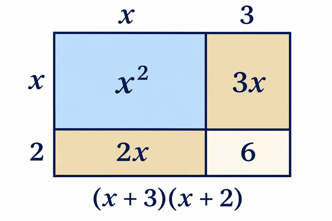
18.8 Multiplying Binomials (FOIL)
Each term in one binomial multiplies each term in the other. . FOIL is a memory aid for four products, while the distributive property explains why the method works.
18.9 Multiplying Polynomials
For larger polynomials, use a table or systematic distribution. . Collect like terms only after writing every product so no middle term is lost.
18.10 Special Polynomial Products
Useful identities include and . Identify the whole expressions playing the roles of a and b. The identities remain valid when those expressions contain coefficients or variables.
18.11 Difference of Two Squares
The product equals because its middle terms cancel. This is a difference of two squares. The sum does not factor into the same pair over the real numbers.
18.12 Squaring Binomials
Squaring a binomial includes a cross term: . It is not . Substituting quickly disproves the incorrect version, while distribution proves the correct identity.
18.13 Dividing Polynomials by Monomials
Divide each numerator term by the monomial denominator, assuming it is nonzero. for . The simplified expression does not remove the original restriction.
18.14 Simplifying Polynomial Expressions
Expand, combine and order terms carefully. . Check the leading term and constant separately; errors often come from the minus sign before the second bracket.
18.15 Polynomial Modeling Problems
A rectangle with sides and has area . Specify a domain making both lengths positive. The polynomial models area only under those geometric restrictions; a negative side length is not viable.
PART 4 · CHAPTER 19
19. Factoring Polynomials
Back to contents ↑19.1 Understanding Factoring
Factoring reverses multiplication by writing an expression as a product. . An expanded polynomial reveals its terms, while factored form often reveals zeros or useful dimensions.
19.2 Greatest Common Factor (GCF)
The greatest common factor combines the greatest numerical factor and the smallest shared exponent of each variable. For and , the GCF is . Factor it before attempting a more specialized pattern.
19.3 Factoring Out a Monomial
Factor as . Divide every term by the extracted factor and verify by distribution. If all leading terms are negative, factoring out a negative GCF can simplify the remaining pattern.
19.4 Factoring Trinomials: x²+bx+c
For , seek integers with sum b and product c. In , 3 and 4 work, giving . If no integer pair works, do not assume the quadratic has no real roots.
19.5 Factoring Trinomials: ax²+bx+c
For , find numbers with product 6 and sum and 1. Split the middle term, , then group to obtain .
19.6 Factoring by Grouping
Group terms to expose a common binomial. . The grouped factors must match exactly; reorder or factor out a negative when needed.
19.7 Difference of Squares
Use . Thus . Both terms must be perfect squares and the operation must be subtraction for this identity.
19.8 Perfect Square Trinomials
Recognize . For , the outer squares are and 25 and the middle term is , so the factorization is .
19.9 Factoring Completely
Factor out the GCF, then inspect the remaining expression repeatedly. . “Completely” depends on the requested coefficient system, typically integer or real factors in the task.
19.10 Relationship Between Factors and Zeros
For a product equal to zero, each real linear factor gives a zero. In , zeros are 2 . A factor’s written constant has the opposite sign from its root.
19.11 Using Factoring to Solve Equations
Set the equation equal to zero before using the zero-product property. From , write , giving . You cannot set individual factors to zero when their product equals a nonzero value.
19.12 Verifying Factored Expressions
Expand the proposed factors and compare every coefficient. produces . A correct constant alone does not verify a factorization; the middle term and leading coefficient must match as well.
19.13 Common Factoring Errors
Do not stop before factoring the GCF or confuse a sum of squares with a difference. If is proposed for , expansion gives the wrong middle term. Verification catches plausible-looking but incorrect pairs.
19.14 EOC-Style Factoring Questions
Factor : extract 3, then recognize . The complete factorization is . If asked for the zero, it is 2; the factor 3 is not an additional zero.
PART 4 · CHAPTER 20
20. Solving Quadratic Equations
Back to contents ↑20.1 What Is a Quadratic Equation?
A quadratic equation has highest variable power two after simplification, with nonzero quadratic coefficient. Its graph-based solution corresponds to intersections or zeros. It may have two, one repeated or no real solutions.
20.2 Quadratic Equation Standard Form
Write with before identifying coefficients. For , use . The sign of b comes from the rearranged equation, not its original position.
20.3 Solving Quadratics by Factoring
For , factor to . Then or . Check both in the original equation and apply any contextual restriction separately.
20.4 Zero Product Property
If a real product equals zero, at least one factor is zero. This justifies solving each factor equation. It does not justify setting in ; first rewrite that equation as a zero product.
20.5 Solving Quadratics Using Square Roots
For , take both square-root possibilities: , so or . The square-root symbol itself gives the principal root; the plus-or-minus arises from solving the squared equation.
20.6 Completing the Square
For , add 9 to both sides: . Then , giving 1 . Half the x-coefficient, then square it, after making the quadratic coefficient one.
20.7 Quadratic Formula
For , use . In , the numerator is and denominator 2, giving 3 and 2. Enclose the full numerator and denominator when entering a calculator.
20.8 Using the Discriminant
The discriminant is . Positive D gives two distinct real roots, zero gives one repeated real root and negative D gives no real roots. Compute D before the square root to catch an unsuitable real-number calculation.
20.9 Number and Type of Solutions
For , D is positive and roots are ±2. For , D is zero and the only distinct root is 2. For , D is negative and no real x satisfies the equation.
20.10 Real and Non-Real Solutions: Conceptual Extension
A negative discriminant leads to complex roots when the number system is extended using . This is a conceptual extension here, not a claim that complex-number calculation is a primary Algebra 1 EOC target. In real-only questions, report no real solution.
20.11 Selecting an Appropriate Solution Method
Use factoring when structure is clear, square roots when a squared expression is isolated, completing the square to expose a vertex, and the quadratic formula for a general quadratic. The discriminant helps predict the real solution count before finishing.
20.12 Solving Quadratic Word Problems
A rectangle has width x and length , with area 40. Solve , giving . Reject as a length and report width 5 and length 8 in the stated units.
20.13 Projectile Motion and Area Applications
For a height model , ground level means , so . The times are 0 and 4; landing after launch is 4. This simplified model assumes its units and physical conditions are appropriate.
20.14 Checking Quadratic Solutions
Substitute each root into the original equation, especially after squaring or dividing by an expression. If the task asks for time or length, also check feasibility. An algebraic root can be mathematically correct but excluded by the story’s domain.
20.15 Multi-Step Quadratic EOC Practice
For a revenue model , find when revenue is 20: , so . These are input levels, not revenue values. Verify both and interpret whether whole-number counts and model limits permit them.
PART 4 · CHAPTER 21
21. Graphing Quadratic Functions
Back to contents ↑21.1 Understanding Parabolas
The graph of a nondegenerate quadratic function is a parabola with a vertical axis of symmetry. It has one turning point called the vertex. Its opening direction depends on the sign of the quadratic coefficient.
21.2 Quadratic Parent Function
The parent has vertex , axis , domain all real numbers and range . Points at opposite inputs share outputs. Use as reference points.
21.3 Standard Form: y=ax²+bx+c
In , c is the y-intercept and a controls opening and vertical scaling. The vertex is not generally . Use and evaluate the function to locate it.
21.4 Vertex Form: y=a(x-h)²+k
Vertex form shows vertex directly. In , the vertex is and the graph opens upward. Its minimum output is .
21.5 Factored Form: y=a(x-r₁)(x-r₂)
Factored form displays real zeros . For , the symmetry axis is halfway between them at . Evaluate there to obtain the vertex .
21.6 Finding the Vertex
For , compute , then . The vertex is . Both coordinates are required when the question asks for a point.
21.7 Finding the Axis of Symmetry
The vertical symmetry axis is in standard form or in vertex form. Write it as a line equation, not as a single point or the horizontal line .
21.8 Finding X-Intercepts and Y-Intercepts
Set x to zero for the y-intercept, and solve the quadratic with y zero for x-intercepts. The graph can have zero, one or two x-intercepts. Its y-intercept always exists for an unrestricted polynomial function.
21.9 Finding Maximum and Minimum Values
If a is positive, the vertex gives a minimum; if a is negative, it gives a maximum. For , the maximum value is 9 at . State the value and its input according to the question.
21.10 Direction of Opening and Width of a Parabola
Positive a opens upward, negative a downward. Relative to the same scale and parent, larger gives a narrower-looking parabola because outputs change more rapidly away from the vertex. Axis scaling can change visual appearance without changing a.
21.11 Quadratic Transformations
Read inside shifts before outside changes: shifts left 1, reflects across the x-axis, compresses vertically by and shifts up 3. The vertex stays identifiable as .
21.12 Domain and Range
The unrestricted quadratic domain is all real numbers. For , range is ; for , , where k is the vertex output. A context such as projectile time can restrict both domain and practical range.
21.13 Increasing and Decreasing Intervals
An upward parabola decreases to its vertex input h and increases after h. A downward parabola does the reverse. Write intervals using x-values; the vertex’s y-value is not the dividing input.
21.14 Comparing Quadratic Graphs
Compare vertex, opening, scale and intercepts on matching axes. Two quadratics with the same vertex can have different output values away from it. If a question asks which is greater at , evaluate there rather than comparing only maximum or minimum values.
21.15 Writing Quadratic Equations from Graphs
If the vertex is , write . A point gives , so . One known vertex and another distinct point determine this vertical-axis quadratic.
21.16 Quadratic Function Real-World Applications
In , maximum modeled profit is 50 at input 5. Explain what the input measures and restrict it to feasible values. A vertex outside a restricted domain may not be the attainable maximum on that domain.
PART 4 · CHAPTER 22
22. Absolute Value Equations & Functions
Back to contents ↑22.1 Understanding Absolute Value
Absolute value is distance from zero: . Distances are nonnegative. More generally, measures distance between x and a, which explains two possible inputs at a positive specified distance.
22.2 Evaluating Absolute Value Expressions
Evaluate inside first, then take absolute value, then complete outside operations. . An expression containing absolute value can have a negative final result when an outside operation makes it negative.
22.3 Solving Absolute Value Equations
For , solve or , giving 3 . A negative right side gives no solution, and a zero right side gives one branch.
22.4 Identifying Extraneous Solutions
A candidate is extraneous if it fails the original equation or its domain. Before splitting , recognize there is no solution. Always check candidates after transformations that may introduce possibilities, such as squaring.
22.5 Introduction to Absolute Value Functions
The basic absolute value graph is V-shaped because its rule changes slope at the vertex. It is linear on each side but not one linear function across its whole domain. Its vertex is an abrupt corner rather than a quadratic turning curve.
22.6 Graphing y=|x|
For , use when and when . The vertex is , domain all real numbers and range nonnegative. Both arms rise away from the vertex.
22.7 Graphing y=a|x-h|+k
In , the vertex is and arm steepness is . Positive a opens upward, negative a downward. Plot the vertex and one point on each side to avoid drawing a parabola by mistake.
22.8 Vertex of an Absolute Value Graph
For , the vertex is . The inside expression is zero at . This is the most reliable way to check the horizontal shift sign.
22.9 Absolute Value Transformations
The graph shifts right 4 and up 2, then opens downward through x-axis reflection. Its maximum value is 2. Describe transformations from the parent and confirm the result with one nearby input.
22.10 Domain and Range
An unrestricted nonconstant absolute value function has all real inputs. Its range is for positive a or for negative a. If , it becomes the constant function instead of a V.
22.11 Piecewise Interpretation of Absolute Value
Split at the input making the inside expression zero. For , use when and when . Each branch must be paired with its correct interval.
22.12 Absolute Value Real-World Applications
A temperature within 2 degrees of 20 can be modeled by , equivalent to . Distance language helps translate tolerance problems without reversing the endpoints.
22.13 Comparing Absolute Value with Linear and Quadratic Functions
A line has one constant slope, an absolute value graph has two linear arms, and a quadratic has smoothly changing slope. Compare their values or rates on a specified interval. A shared vertex or intercept does not make their growth patterns identical.
22.14 Multi-Step EOC Questions
Solve : subtract 3, divide by 2 and obtain . Then or . Substitute both into the original expression, which returns 11 in each case.
PART 4 · CHAPTER 23
23. Exponential Functions, Growth & Decay
Back to contents ↑23.1 Introduction to Exponential Functions
An exponential function places the variable in the exponent. In , use , and typically for a nonconstant model. Equal input increments multiply outputs by a constant factor.
23.2 Linear vs. Exponential Growth
Linear growth adds a constant amount each period; exponential growth multiplies by a constant factor. Starting from 100, adding 10 gives 110 then 120, while growing 10% gives 110 then 121. They agree after one step but then separate.
23.3 Exponential Function Form: y=abˣ
In , a is the value at and b is the one-unit factor. For , the initial value is 50 and each step multiplies by 1.2. The time unit must be stated in an applied model.
23.4 Identifying Initial Value and Growth Factor
A table with outputs 12, 18, 27 at inputs 0, 1, 2 has initial value 12 and factor 1.5. The model is . If the input increments differ from one, the consecutive-output ratio is not automatically the per-unit factor.
23.5 Exponential Growth
With positive initial amount and factor , the model grows. A 6% increase uses factor 1.06, not 0.06 or 6. For a USD 200 starting value after 2 periods, .
23.6 Exponential Decay
With positive initial amount and factor between 0 and 1, the model decays. A 15% loss retains 85%, so use . The amount stays positive in the ideal exponential model rather than becoming negative after enough steps.
23.7 Growth and Decay Rates
Growth rate r gives factor ; decay rate r gives factor when r is a positive loss rate. Factor 0.92 means 8% decay per period. Convert percentages to decimals before substituting.
23.8 Creating Exponential Models from Tables
For equal one-unit steps, divide consecutive outputs to find b, then use a known pair to find a. If are given, and . Verify the model against every supplied pair.
23.9 Writing Exponential Equations from Context
A machine worth USD 8,000 loses 12% each year, so for nonnegative years t. State the constant-percentage assumption. Do not subtract USD 960 each year; that would be a different linear depreciation model.
23.10 Graphing Exponential Functions
Plot the y-intercept and several values on either side of zero, then sketch a smooth curve. For , useful points are . It approaches but does not meet for finite real x.
23.11 Horizontal Asymptotes and End Behavior
For with nonzero a and no vertical shift, is the horizontal asymptote. In , the horizontal asymptote is . “Approaches” does not mean reaches the asymptote at a finite input.
23.12 Domain and Range of Exponential Functions
For a positive a and positive base not equal to one, the unrestricted real domain is all real numbers and range is positive. A negative a reflects outputs below zero. Applied time models often use only or discrete whole periods.
23.13 Comparing Linear, Quadratic and Exponential Growth
On a long positive-input horizon, exponential growth with factor greater than 1 eventually dominates polynomial growth. On the actual interval in a question, calculate or compare values. A large initial linear amount can stay larger for many periods.
23.14 Population Growth Problems
A population of 500 growing 3% annually follows under a constant-rate assumption. After 2 years it is 530.45 in the model. Round people only when the question requires an estimated whole population.
23.15 Depreciation and Decay Problems
A substance retaining 70% each hour has model . Its loss rate is 30%, not 70%. After two hours it retains 49% of its initial amount, because the second loss applies to the remaining quantity.
23.16 Exponential Modeling Practice
Starting at 80 with values 100 and 125 one and two periods later gives factor 1.25 and model . To predict the next period, calculate 156.25. Explain the 25% increase and distinguish a model from a guaranteed real-world outcome.
PART 4 · CHAPTER 24
24. Financial Literacy & Nonlinear Modeling
Back to contents ↑24.1 Mathematical Modeling of Financial Situations
Identify principal, rate, time unit, compounding frequency and any deposits or withdrawals. A model assuming no additional cash flows is unsuitable for an account receiving monthly deposits unless those flows are included separately. Compare options over the same duration.
24.2 Simple Interest Formula
Simple interest is and total amount with consistent annual rate and years. For , interest is USD 150 and amount USD 1,150. Interest and final balance are different quantities.
24.3 Compound Interest Formula
Compound interest with n periods per year is , assuming a fixed nominal annual rate and no cash flows. For USD 1000 at 6% compounded twice yearly for one year, .
24.4 Growth of Savings Accounts
Interest credited to savings can itself earn later interest. With annual compounding at 4%, USD 500 becomes USD 520 after one year and USD 540.80 after two. Account fees, changing rates or deposits require a modified model.
24.5 Investment Value Over Time
The formula gives a modeled value, not a promise of investment return. A constant annual growth assumption may be useful in a mathematics question, while real investments fluctuate. Retain full precision during the calculation and round currency at the requested final step.
24.6 Comparing Simple and Compound Interest
For the same positive principal and annual rate over multiple annual periods, compound growth adds interest on earlier interest while simple interest adds the same amount each year. At USD 1000 and 10% for 2 years, simple gives USD 1200 and annual compound gives USD 1210.
24.7 Exponential Growth in Financial Models
Annual compound growth is exponential in time: . A negative annual change can model depreciation instead. Explain whether the amount is multiplied by a factor each period or increased by a fixed dollar amount.
24.8 Interpreting Rates and Time Periods
A 12% nominal annual rate compounded monthly uses 0.01 per month and 12t periods over t years. Do not apply 12% every month. Keep the rate period and exponent’s period count aligned.
24.9 Comparing Financial Options
Compare final balances under identical principal, duration and cash-flow assumptions. A higher advertised nominal rate can be offset by fees or different compounding. In a constrained exam problem, use only the provided terms and state the conclusion within those assumptions.
24.10 Nonlinear Modeling with Graphs and Tables
A table’s ratios can reveal compound growth and its differences can reveal simple-interest growth. Graphs show how the gap develops over time. Choose a viewing range that makes the relevant comparison visible without implying a constant difference where none exists.
24.11 Multi-Step Application Questions
A USD 2000 balance earns 5% annually for 2 years, then a USD 100 withdrawal occurs. Compute . If the withdrawal happens earlier, it changes later interest, so the event order must be modeled explicitly.
24.12 Mixed Reporting Category 3 Practice Test
Questions 33–48 of each complete form cover nonlinear relationships. Practise polynomial structure, quadratic roots and graphs, absolute value, exponentials and finance. Review both the chosen model and the arithmetic; correct calculation cannot rescue an unsuitable relationship.
PART 5 · CHAPTER 25
25. Complete Algebra 1 EOC Formula Sheet
Back to contents ↑25.1 Official Florida Algebra 1 EOC Reference Sheet
Use the official reference sheet provided through your school’s sample test to learn its layout. Do not assume it contains every identity in this chapter. The searchable cards below intentionally include additional study relationships, with their conditions stated.
25.2 Laws of Exponents
For compatible nonzero bases, multiply powers by adding exponents, divide by subtracting exponents and raise a power by multiplying exponents. Remember and for . The operation between expressions determines the applicable rule.
25.3 Radical Rules
For nonnegative a,b, and for real a. Addition has no comparable square-root distribution rule. Simplify perfect-square factors before combining like radicals.
25.4 Algebraic Properties
Distributivity gives ; commutativity and associativity allow reordering and regrouping addition or multiplication. They do not permit arbitrary rearrangement of subtraction or division. Name the property when justifying an equivalence.
25.5 Linear Equation Formulas
Use slope-intercept , point-slope or standard according to available information. Vertical lines require . An equation’s form can change while its solution set remains the same.
25.6 Slope and Rate of Change Formulas
Slope and average rate both use output change divided by input change. For a line, the rate is constant; for a nonlinear function, specify the interval. The denominator must be nonzero and the units are output units per input unit.
25.7 Parallel and Perpendicular Line Rules
Parallel nonvertical lines have equal slopes; perpendicular nonvertical, nonhorizontal lines have negative reciprocal slopes. Distinct intercepts distinguish parallel lines from identical lines. Handle horizontal/vertical pairs separately instead of dividing by zero.
25.8 Linear Inequality Rules
Adding or subtracting the same quantity preserves inequality direction. Multiplying or dividing by a negative reverses it. Strict comparisons exclude boundaries; inclusive comparisons include them. A test point provides a fast independent check of the final region.
25.9 Systems of Equations Methods
Graphing identifies intersections, substitution replaces one variable with an equal expression, and elimination combines equations to cancel a variable. A contradiction signals no solution; an identity signals dependent equations, subject to the original relationship.
25.10 Polynomial Identities
Recall , and . Verify the middle coefficient rather than recognizing only the outside squares.
25.11 Factoring Formulas
Extract the GCF first, then inspect trinomial, grouping or square patterns. For monic , the two factor constants add to b and multiply to c. Expand your answer to verify every term.
25.12 Quadratic Formula
The quadratic formula applies to with . Both branches use the same full denominator 2a. Enter negative coefficients in parentheses to preserve the square in .
25.13 Discriminant Formula
Use to determine the real-root count before solving. means two distinct roots, a repeated root and no real roots. A negative D is not a calculator malfunction.
25.14 Vertex and Axis of Symmetry Formulas
For standard form, the vertex input and axis are determined by and vertex output . For vertex form, read h,k directly. The axis is the line , while the vertex is the point .
25.15 Exponential Growth and Decay Formulas
Use for repeated growth and for repeated loss, with rates and time measured per matching period. A 20% decay retains 80%, so its factor is 0.8.
25.16 Simple and Compound Interest Formulas
Simple interest is ; compound amount is . The latter assumes no additional deposits or withdrawals and a constant nominal rate. Report whether the question asks for interest earned or final amount.
25.17 Statistical Formulas and Relationships
Mean is sum divided by count, range is maximum minus minimum, IQR is , relative frequency is relevant count divided by its specified total, and residual is observed minus predicted. Name denominators and variables before computing.
25.18 Provided Formulas vs. Additional Relationships Worth Learning
A supplied formula does not replace understanding of its symbols and conditions. Learn exponent laws, sign rules, model recognition and interpretation even if a related expression appears on the reference sheet. Use the full study cards for revision, not as a claim about permitted exam materials.
25.19 Printable Two-Page Formula Cheat Sheet
Download the two-page formula sheet in Chapter 36, cover its equations and recall each from its label. Then explain one condition of use and solve a quick example. Printing a sheet is useful only when it supports active retrieval and application.
Searchable formula reference
30 formula cards
Multiply every term; signs remain part of each term.
For the quotient, a must be nonzero.
Apply within the real domain where both expressions are defined.
; a negative exponent means reciprocal.
Reduce ; check the real domain for even roots.
For real square roots, a,.
Do not assume x is nonnegative unless stated.
Distinct x-values; vertical slope is undefined.
m is rate and is the y-intercept.
Uses a known point and a finite slope.
A and B are not both zero for a line.
Distinct parallel lines; reciprocal rule excludes horizontal/vertical pairs.
; include output units per input unit.
Constant ratio at nonzero inputs and graph through the origin.
Reverse the comparison when multiplying or dividing by a negative.
gives a unique solution for and .
The operation must be subtraction.
Include the middle product with the matching sign.
The constants must match both sum and product.
For with .
Positive: two real roots; zero: repeated root; negative: no real roots.
Vertex ; symmetry axis .
gives a minimum, a maximum.
Real zeros are r₁,r₂; midpoint is the symmetry input.
Requires ; gives one branch.
; match the time period to the factor.
r is a positive decimal gain or loss rate, respectively.
Annual rate and time in years; no added cash flows.
Nominal annual rate, n compounds per year; no cash flows.
; residual is observed minus predicted.
Algebra recall flashcards
Recall the rule and its conditions before revealing the answer.
When does the inequality flip?
When you multiply or divide both sides by a negative.
Why two square-root branches?
A positive square can come from a positive or a negative original value.
What does a factor of 0.85 mean?
85% remains each period, so the positive starting amount decays by 15%.
What makes a system solution valid?
It satisfies every original condition and the contextual domain.
Which denominator for a conditional rate?
The total for the specified condition or subgroup.
What proves a factorization?
Expanding reconstructs every coefficient of the original expression.
How do horizontal shifts work?
f(x-h) shifts the graph right by h; find the input making the inside zero.
What is a residual?
Observed output minus the model’s predicted output.
What does a negative discriminant mean?
The quadratic has no real roots or x-intercepts.
Does correlation prove causation?
No. Confounding, sample design and other explanations must be considered.
PART 5 · CHAPTER 26
26. Algebra 1 EOC Common Mistakes
Back to contents ↑26.1 Sign Errors with Negative Numbers
Keep subtraction and a negative input separate. , while and . Parentheses show which quantity is squared and protect signs during calculator entry.
26.2 Order of Operations Mistakes
Multiplication and division share priority and run left to right, as do addition and subtraction. In , the answer is 18. Treating multiplication as always before division changes the expression incorrectly.
26.3 Distributive Property Errors
A multiplier outside brackets applies to every term. , not . Draw distribution arrows or write separate products if the outer negative is easy to overlook.
26.4 Combining Unlike Terms
Only terms with matching variable parts combine by adding coefficients. stays two terms. Multiplication follows a different rule: .
26.5 Incorrect Exponent Rules
Do not apply a product rule to a sum: is not . Also is not . Identify the full base and operation before manipulating exponents.
26.6 Radical Simplification Errors
The root of a sum does not split: , while . Extract square factors from products instead, and remember absolute value when simplifying the square root of a variable square.
26.7 Equation-Solving Errors
Every equation operation must preserve equality on both sides. From , subtract 3 from both sides before dividing by 2. Dividing just the term on the left while retaining the rest unscaled is invalid.
26.8 Inequality Sign Reversal Mistakes
Reverse the inequality only when multiplying or dividing both sides by a negative. From , obtain . Subtracting a positive or negative number alone does not trigger reversal.
26.9 Confusing Slope and Intercepts
In , slope is and y-intercept is 5. The zero is , a third feature. Label the units and location of each so a correct number is not used to answer the wrong question.
26.10 Incorrect Shading of Inequalities
Choose shading with a point not on the boundary. For , the origin fails, so shade the opposite side. A boundary style error and a shading error are separate checks.
26.11 Systems of Equations Calculation Errors
When multiplying an equation for elimination, multiply every term including the constant. Keep variable order aligned, then substitute the result into both original equations. A pair that passes only one is incomplete.
26.12 Polynomial Multiplication Errors
Each term in one factor multiplies every term in the other. . Omitting the middle products produces the wrong polynomial even when the first and last terms look right.
26.13 Factoring Errors
Check the sum as well as the product of trinomial constants. For , both constants must be negative: . Extract any common factor before deciding the expression is fully factored.
26.14 Quadratic Formula Sign Errors
Use the sign of b from standard form. If , then and . Place the entire numerator over 2a; dividing only the square-root term is a different expression.
26.15 Incorrect Graph Interpretation
Read axis scales, open endpoints and the requested feature. A graph below the x-axis can still be increasing. Negative outputs and a negative rate of change describe different things.
26.16 Exponential Growth vs. Decay Confusion
A 10% loss uses factor 0.9, not . A 10% gain uses 1.1, not 0.1. Write “retain 90%” or “become 110%” before converting to the multiplication factor.
26.17 Statistics and Data Interpretation Mistakes
Conditional percentages require the relevant subgroup denominator, not automatically the grand total. A box plot shows quartile summaries, not every individual observation. Distinguish a sample association from a causal conclusion.
26.18 How to Check and Correct Your Answers
Use a different check from the original method: substitute into an equation, expand a factorization, inspect units or test a feasible point. Record the first error and a prevention cue, then solve a fresh example to show the correction transfers.
PART 5 · CHAPTER 27
27. Algebra 1 EOC Quick Review & Cheat Sheet
Back to contents ↑27.1 All Essential Algebra Concepts in One Place
Organize recall around three questions: what structure is present, which operation preserves it, and what does the result mean? Move between expression, equation, graph and context. Use the short revision sheet as a retrieval checklist rather than rereading it passively.
27.2 Important Algebraic Rules
Keep signs attached to terms, distribute across whole brackets, combine only like terms and respect nonzero denominators. Before canceling, ask whether you are removing a factor from a product or incorrectly canceling across addition.
27.3 Linear Relationships Quick Review
A line has constant rate; equations give exact conditions; inequalities describe permitted sets; and systems require simultaneous satisfaction. Check intercepts, slope units, boundary inclusion and all contextual restrictions.
27.4 Nonlinear Relationships Quick Review
Recognize polynomial degree, factored zeros, quadratic vertex and exponential multiplier. Select a method from the structure rather than forcing every nonlinear problem into the quadratic formula. Absolute value introduces distance and two possible branches.
27.5 Functions and Graphs Quick Review
A function gives one output per allowed input. Read domain, range, zeros, extremes and rates from the requested representation. Transformation signs inside the input behave differently from shifts added outside.
27.6 Statistics Quick Review
Sort data before finding a median, use the correct total for a conditional rate, preserve paired observations in scatter plots and compute residual as observed minus predicted. Explain a data result in the context of the measured population and units.
27.7 Important Equations and Formulas
Recall slope, line forms, exponent laws, quadratic formula, vertex input, exponential growth and interest relationships. State when each formula is valid. The formula cards below include conditions so memorization does not become mechanical substitution.
27.8 Common Graph Shapes
Match straight lines to linear models, smooth U-shapes to quadratics, V-shapes to absolute value and repeated-factor curves to exponentials. Scale, shifts and restrictions alter appearance, so verify using an equation or representative coordinates.
27.9 How to Recognize Question Types
Look for the task verb: simplify changes an expression’s form, evaluate finds an output, solve finds permitted inputs, graph represents a set and interpret explains a feature. Underline what the requested answer actually represents before calculating.
27.10 Fast Problem-Solving Methods
Use structure to reduce work: isolate a squared expression before using a general formula, eliminate aligned coefficients in a system, or use an intercept when it is immediately available. Efficiency should remove unnecessary work without skipping conditions or checks.
27.11 Last-Minute Memory Aids
Remember “same base, multiply: add exponents,” “negative divisor: flip inequality,” and “residual: actual minus predicted.” Attach one worked example to each cue. A phrase without a mathematical condition is easy to misuse.
27.12 Printable Final Revision Sheet
The final-review PDF in Chapter 36 condenses the three categories and key checking habits onto one page. Use it on the final day to retrieve known methods. Return to a chapter whenever you cannot explain one of its prompts confidently.
PART 6 · CHAPTER 28
28. Algebra 1 EOC Worked Examples
Back to contents ↑28.1 Beginner-Level Worked Examples
Solve : subtract 5 to get , divide by 2 to get , then check . This three-stage pattern—setup, valid operations, original check—scales to more complicated tasks.
28.2 Intermediate-Level Worked Examples
Solve : expand to , subtract , then add 6 to obtain . Substitution gives 27 on both sides. The negative constant inside the bracket must also be multiplied by 3.
28.3 Advanced-Level Worked Examples
A rectangle has perimeter 26 and area 40. Let sides be x and y: . Substituting gives , so sides are 5 and 8. Both assignments describe the same rectangle.
28.4 Algebraic Expression Examples
Simplify : expand to , collect x-terms to and constants to . The result is . A check at gives zero in both forms.
28.5 Equation and Inequality Examples
Solve : distribute to , subtract 6, then divide and reverse the sign. The result is . Testing works; testing 0 fails.
28.6 Graph Interpretation Examples
For , the maximum is 9 at , the y-intercept is 5, and zeros satisfy , giving and 5. These features create a consistent sketch.
28.7 Function Comparison Examples
Compare with table values under a linear assumption. The slopes are 3 and 2, starting values 2 and 5. Solving shows equality at .
28.8 Systems of Equations Examples
For and , add to obtain , hence and . Substitution checks both 9 and 3. The output is the ordered pair .
28.9 Polynomial and Factoring Examples
Factor : extract 2, then factor as . Final form is . Expansion reconstructs each original coefficient.
28.10 Quadratic Equation Examples
Solve . The discriminant is ; the quadratic formula gives , so roots are 2 . Factoring as independently verifies them.
28.11 Exponential Modeling Examples
A USD 500 item loses 20% annually. After 3 years, . The loss is applied to each remaining balance, so subtracting USD 100 three times would incorrectly give the linear result 200.
28.12 Statistics and Data Analysis Examples
A data point is and the fitted line is . Prediction at is 13, so residual is 2. The observation lies above the line. This does not establish that changing x causes y to increase.
28.13 Multi-Step Real-World Problems
A club pays USD 80 fixed cost and USD 4 per ticket sold; revenue is USD 12 per ticket. Profit is . To earn at least USD 40, solve , giving at least 15 whole tickets.
28.14 Error Analysis with Corrections
A student writes . Correct by expanding . The missing term is . Testing exposes the error immediately: the original is zero, while the proposed expression is 32.
28.15 Detailed Step-by-Step Explanations
For each solution, identify the model, show equivalent steps and verify the original conditions. In a word problem, end with units and a viable interpretation. Read the diagnostic’s full keys to compare this structure across all response types.
PART 6 · CHAPTER 29
29. Topic-Wise Algebra 1 EOC Practice Questions
Back to contents ↑29.1 Algebraic Expressions Quiz
Select Expressions in the practice lab to test interpreting terms and rearranging formulas. Before checking, name the requested operation. For a missed item, compare your first transformation with the explanation, then expand or substitute to verify the correction.
29.2 Exponents and Radicals Quiz
Choose Exponents and radicals for rational powers, equivalent powers and root operations. State any nonzero or real-root restrictions. If an answer differs, determine whether the error came from the exponent law, radicand simplification or final response entry.
29.3 Functions and Function Notation Quiz
Choose Functions to practise evaluating, identifying valid relations and interpreting domains or outputs. Label input and output before calculation. Distinguish a request for from a request to find x when .
29.4 Function Transformations Quiz
Choose Transformations to connect a changed function rule with its shifted or reflected graph. Find the parent and vertex or anchor point first. Use a nearby input as a check on the direction and scale.
29.5 Data Analysis and Statistics Quiz
Choose Statistics for centers, spread, displays and conditional frequencies. Write the denominator or reference group before calculating. Review why a selected representation or summary fits the data rather than memorizing the numerical result alone.
29.6 Linear Equations Quiz
Choose Linear equations for balancing operations, literal equations and interpreting solutions. Substitute your candidate into the original equation. If variables cancel, classify the remaining statement as true or false before reporting a solution count.
29.7 Linear Inequalities Quiz
Choose Inequalities for direction reversal, boundary style and point tests. Verify a point from the proposed set. A selected shading region must satisfy the original condition, including whether equality is permitted.
29.8 Slope and Graphing Quiz
Choose Slope and graphing for rates, line equations, intercepts and perpendicular directions. Read the axis units and use consistent coordinate order. Verify a line equation with a second point.
29.9 Systems of Equations Quiz
Choose Systems to practise intersection, substitution, elimination and model construction. Save an ordered pair rather than only one variable. Check both original equations and any whole-number restrictions.
29.10 Systems of Inequalities Quiz
Choose Constraints for feasible regions, budget limits and included boundaries. List every inequality and test the candidate in all of them. Explain which condition excludes a point when it is not feasible.
29.11 Scatter Plots and Linear Models Quiz
Choose Linear models for scatter patterns, predictions, residuals and association. State the units and observed input range. A prediction outside that range deserves extra caution, and correlation alone does not prove causation.
29.12 Polynomials Quiz
Choose Polynomials for addition, multiplication and monomial division. Keep like powers aligned and preserve original denominator restrictions. Use distribution or a coefficient check to verify an expanded result.
29.13 Factoring Quiz
Choose Factoring to practise GCF, trinomial and special-product structure. Expand your chosen factors before checking. The correct leading and constant terms are not enough if the middle coefficient differs.
29.14 Quadratic Equations Quiz
Choose Quadratic equations for factorization, square-root methods and discriminants. Set the equation to zero before choosing coefficients. Check every root and distinguish two distinct roots from one repeated root.
29.15 Graphing Quadratics Quiz
Choose Quadratic graphs for vertex, zeros, range and model interpretation. Read the question’s requested feature carefully. A maximum output, its input and the vertex point are related but different answers.
29.16 Absolute Value Functions Quiz
Choose Absolute value for distance equations and V-shaped graphs. Isolate the absolute value before splitting cases. A negative isolated right side means no solution rather than two automatically generated candidates.
29.17 Exponential Functions Quiz
Choose Exponentials for factors, repeated percentage change and graph features. Translate a loss rate into the retained factor. Check the period unit before using a table ratio or exponent.
29.18 Financial Mathematics Quiz
Choose Finance to compare simple and compound models and interpret financial parameters. Align annual rates with compounding periods. Separate final balance from interest earned and state the no-extra-cash-flow assumption when relevant.
29.19 Mixed EOC Review Quiz
Use Mixed applications to generate a short shuffled set spanning the available question bank. A topic filter may contain fewer items than the chosen cap; the interface shows the actual number loaded. Use a fixed complete form for the balanced category design.
29.20 Full Answer Keys and Worked Solutions
Every original item has its answer and worked steps in the on-page review and corresponding PDF. Attempt first, then inspect the earliest difference in method. Copying a key is not evidence of independent performance; reattempt missed items after a delay.
PART 6 · CHAPTER 30
30. Algebra 1 EOC Full-Length Practice Tests
Back to contents ↑30.1 Diagnostic Practice Test — No. 0
Begin with Diagnostic 0 to identify current strengths and gaps. Work without opening explanations, save every attempt and finish for category and item feedback. The same complete diagnostic is readable without JavaScript below and downloadable with its key.
30.2 Practice Test 1 — Foundation Level
Practice 1 emphasizes familiar structures and clean representations. It is still a 48-item mixed form across all three categories. “Foundation” describes the study emphasis, not a calibrated official difficulty or a guaranteed achievement level.
30.3 Practice Test 2 — Intermediate Level
Practice 2 varies values and contexts so you must transfer the method rather than recall a diagnostic answer. Explain at least one key step for each missed topic. Compare recurring error types, not just the total percentage.
30.4 Practice Test 3 — Mixed Difficulty
Practice 3 combines routine work with additional reasoning. Watch transitions from a story to an equation and from a solution to a feasible interpretation. The fixed form is independent practice, not adaptive testing.
30.5 Practice Test 4 — Advanced Application
Practice 4 includes more linked decisions in selected tasks. Leave enough time to verify signs, domains and units after the main calculation. A longer prompt does not always require a longer method if the structure is recognized.
30.6 Practice Test 5 — Final EOC Simulation
Use Practice 5 as a fresh final rehearsal, with your permitted study calculator and a distraction-free session. Its 48 questions do not reproduce the state interface, adaptive scoring or official reference sheet. Review errors before deciding what to revisit.
30.7 Multiple-Choice and Technology-Enhanced Question Practice
The lab includes single-choice, multi-select, numeric, coordinate and statement-completion responses. These practise important response decisions but are not a replica of every TDS interaction. Use the school’s sample platform for drag, hot-text and graph-entry familiarity.
30.8 Full Answer Keys
Each form’s PDF ends with a full key and worked explanations. The browser report displays the same source answers after finishing. Keep the key covered during an independent attempt, then annotate the method that needs repair.
30.9 Detailed Solution Explanations
Solutions show setup, mathematical reasoning and a result check or interpretation. Read them as explanations rather than answer codes. If your valid alternative method differs, verify it satisfies the original problem before assuming it is wrong.
30.10 Practice Test Score Reports
Reports show local points, unanswered items and category accuracy. Each item earns one point; multi-select is all-or-nothing. These percentages describe this practice set only and are not converted to a B.E.S.T. scale score.
30.11 Benchmark-Wise Performance Analysis
The report links missed items to their benchmark codes and study chapters. Several codes may be connected to one task because the reasoning overlaps. A single item is insufficient evidence of complete mastery or failure of a benchmark.
30.12 Personalized Improvement Recommendations
Start with the category having the lowest practice accuracy, then inspect the first wrong decision in each item. Read that chapter, solve a related fresh task and return to mixed work. A recommendation is a next study step, not an official diagnosis.
30.13 Reattempting Missed Questions
After finishing, use Reattempt missed questions to create a set from incorrect or unanswered items. Your earlier report is replaced when the new attempt begins. For stronger retrieval practice, wait before retrying and avoid reading the key immediately beforehand.
Choose a complete 48-question form
Read all diagnostic questions and worked solutions
These 48 original questions are also available as a PDF. Each practice item is worth one local point; multi-select requires all correct selections and no incorrect selections.
Question 1 · Exponents and radicals
Evaluate 27 raised to the power .
Show answer and reasoning
Answer: 9
A denominator of 3 indicates a cube root.
The cube root of 27 is 3; square it.
The result is 9. The positive base makes the real rational power unambiguous.
Question 2 · Exponents and radicals
For , simplify () / . Which expression is equivalent?
4x
x⁴
x⁸
x⁷
Show answer and reasoning
Answer: x⁴
Multiplication of equal bases adds exponents: .
Division subtracts 2, leaving exponent 4.
The original nonzero restriction remains.
Question 3 · Exponents and radicals
Simplify . Enter the coefficient of .
Show answer and reasoning
Answer: 9
The first root is .
The second is .
Add like radical coefficients: 9.
Question 4 · Expressions
A model gives cost in dollars for v visits. What does 30 represent?
The charge per visit
The number of visits
The total after every possible visit count
The one-time starting charge
Show answer and reasoning
Answer: The one-time starting charge
The constant term is independent of the visit count.
At the modeled cost equals the constant.
The coefficient of v, not the constant, is the charge per visit.
Question 5 · Expressions
Rearrange to isolate , assuming .
Show answer and reasoning
Answer:
Divide both sides by 3w.
The full product 3w is the denominator.
The nonzero assumption makes the division valid.
Question 6 · Functions
A table has x-values 0, 1, 2 and y-values 3, 6, 12. Which function type could model the table?
Absolute value with vertex at
Linear
Exponential
Constant
Show answer and reasoning
Answer: Exponential
Equal x-steps multiply y by 2.
The differences are not constant; the common ratio is 2.
The exponential model is : each unit increase in x doubles the preceding output.
Question 7 · Functions
A delivery cost is . Find , in dollars.
Show answer and reasoning
Answer: 13
Substitute input 4 for x.
Calculate .
The output is 13 dollars; x is the delivery input, not the output.
Question 8 · Functions
The modeled height is . Find average rate of change from to .
Show answer and reasoning
Answer: 4
and .
Divide their output difference by 3-1.
height units per time unit.
Question 9 · Functions
Compare with (). Select all true statements.
f has a larger value at every nonnegative input
The two functions have the same initial value
f has the larger value at
g has the larger value at
Show answer and reasoning
Answer: f has the larger value at ; g has the larger value at
At 0, , .
At 3, , .
The comparison changes with the input; neither is always larger.
Question 10 · Finance
Account 1 earns interest on its original principal only, adding the same dollars each year. Which model describes its balance?
Exponential decay
Linear simple-interest growth
Exponential compound-interest growth
Quadratic growth
Show answer and reasoning
Answer: Linear simple-interest growth
The interest amount is fixed because it uses only the initial principal.
A fixed addition per year produces a linear balance.
Compound interest would multiply the changing balance instead.
Question 11 · Transformations
If and , how is the graph shifted?
Right 3 units
Left 3 units
Up 3 units
Down 3 units
Show answer and reasoning
Answer: Right 3 units
The new input equals zero at .
The parent vertex moves from to .
A subtraction inside the input shifts the graph right.
Question 12 · Statistics
Sample 1 records paired shoe sizes and heights for students. Which display is appropriate for these bivariate numerical data?
One histogram of transport categories
Pie chart of a continuous pair
One box plot that merges both units
Scatter plot
Show answer and reasoning
Answer: Scatter plot
There are two numerical measurements per student.
Keep the paired observations together.
A scatter plot displays numerical association; a single histogram cannot show the pairing.
Question 13 · Statistics
In sample 1, waiting times are strongly right-skewed with a very large outlier. Which summaries best resist that outlier?
Maximum and mean
Mode and total
Median and interquartile range
Mean and range
Show answer and reasoning
Answer: Median and interquartile range
The extreme value can substantially move the mean and standard deviation.
Median uses central ordering and IQR uses the middle half.
They provide a resistant center-and-spread pair.
Question 14 · Statistics
A table for class 1 has 18 bus riders, 12 walkers and 9 early bus riders. How many bus riders are not early?
Show answer and reasoning
Answer: 9
The bus total includes early and not-early riders.
Subtract 9 from 18.
The remaining joint cell is 9; walkers belong to a different row.
Question 15 · Statistics
A survey records 6 early cyclists, 9 late cyclists, 3 early drivers and 12 late drivers. Which group has the larger early-arrival proportion?
Cyclists
Drivers
Equal proportions
Cannot compare because the totals are equal
Show answer and reasoning
Answer: Cyclists
Cyclists: %.
Drivers: %.
Compare the conditional rates, not just the total number of early travelers.
Question 16 · Functions
For model 1, which rule is quadratic?
|x|
Show answer and reasoning
Answer:
A quadratic polynomial has highest variable exponent 2.
The variable is not in an exponent or absolute value.
Its nonzero leading coefficient gives a parabola.
Question 17 · Linear equations
A club pays a $9 fee and $3 per participant, totaling $18. How many participants are there?
Show answer and reasoning
Answer: 3
Write .
Subtract 9 and divide by 3.
; substituting gives the stated total.
Question 18 · Slope and graphing
A line has y-intercept 3 and passes through . Choose its equation.
Show answer and reasoning
Answer:
Slope is .
The intercept is 3.
Substitute the supplied point to verify both features.
Question 19 · Slope and graphing
Find the slope of a line perpendicular to .
3
Show answer and reasoning
Answer:
Perpendicular nonvertical lines have negative reciprocal slopes.
The original slope is 3.
The negative reciprocal is , whose product with 3 is .
Question 20 · Slope and graphing
For , find its x-intercept as an ordered pair.
Show answer and reasoning
Answer: 3,0
Set y to zero.
, so .
The ordered pair is , not .
Question 21 · Slope and graphing
A tank starts with 30 liters and loses 3 liters each minute until empty. What is the largest viable time in minutes?
Show answer and reasoning
Answer: 10
Model with .
Set .
The viable time domain is ; the line beyond it predicts negative water.
Question 22 · Inequalities
A student's budget requires after rearrangement. Which solution set is correct?
Show answer and reasoning
Answer:
Subtract 6 to get .
Divide and reverse the comparison.
The result is ; the boundary is excluded.
Question 23 · Inequalities
Tickets cost $3 for adults and $2 for children. A budget of at most $30 is available. Which inequality models it?
Show answer and reasoning
Answer:
Multiply each ticket count by its price.
Add both costs and compare with the budget.
At most permits equality, so use ≤.
Question 24 · Inequalities
How should the solution to be graphed?
Solid boundary; shade above
Dashed boundary; shade below
Solid boundary; shade below
Dashed boundary; shade above
Show answer and reasoning
Answer: Dashed boundary; shade above
The excluded boundary line is ; equality is not permitted by >.
Strict > excludes the boundary, so it is dashed.
Larger y-values lie above the boundary.
Question 25 · Systems
Solve and . Enter x,y.
Show answer and reasoning
Answer: 6,3
Add the equations: .
Then and .
Check both original equations: , and . Both hold.
Question 26 · Constraints
For , , , which describes the feasible region?
The triangle with all three boundary sides excluded
The first-quadrant triangle including its three boundary sides
Only points above the diagonal in every quadrant
The entire first quadrant
Show answer and reasoning
Answer: The first-quadrant triangle including its three boundary sides
The axes restrict the region to nonnegative coordinates.
The line connects and .
The ≤ sign includes the line and the side toward the origin.
Question 27 · Constraints
A shop makes whole items x,y with , , , . Is feasible?
Yes; both resource constraints and count restrictions hold
No; it exceeds the item limit
No; it exceeds the resource limit
No; negative counts are required
Show answer and reasoning
Answer: Yes; both resource constraints and count restrictions hold
Total items: .
Resource use: .
Both counts are nonnegative integers.
Question 28 · Slope and graphing
Compare with a linear table for , . Which has larger slope?
f
Equal slopes
Neither has a slope
g
Show answer and reasoning
Answer: g
The slope of f is 2.
The table rate is .
Thus g has the larger rate, regardless of the different intercepts.
Question 29 · Linear models
A fitted model predicts . Find predicted y at .
Show answer and reasoning
Answer: 9
Substitute into the line.
Calculate ; the predicted output is 9.
This is a model prediction, not a guaranteed individual outcome.
Question 30 · Linear models
Scatter plot 1 shows paired points close to a decreasing straight line, with small residuals of both signs. Which interpretation fits?
Proof that x causes y to decrease
Strong negative linear association
Weak positive linear association
No relationship of any kind
Show answer and reasoning
Answer: Strong negative linear association
The pattern decreases as x grows, so direction is negative.
Small residuals around a line indicate a close linear fit.
This establishes association, not causation.
Question 31 · Linear models
For fitted line , observations at ,2,3 have y-values 6,6,10. Which residual sequence is correct?
1, , 1
, 1,
3, 3, 7
0, 0, 0
Show answer and reasoning
Answer: 1, , 1
The predicted values at the three supplied inputs are 5, 7 and 9. Compare each observation with its matching prediction.
Residual is observed minus predicted.
The residuals are 1, and 1, straddling zero.
Question 32 · Systems
For equation pair and . How many solutions exist?
Exactly one solution
Infinitely many points on one shared line
Every ordered pair
No solutions
Show answer and reasoning
Answer: No solutions
Divide the second equation by 2.
It becomes , while the first line is . Equal slopes and unequal intercepts make them parallel.
Distinct parallel lines never intersect.
Question 33 · Polynomials
Expand . Which is correct?
Show answer and reasoning
Answer:
Multiply all four term pairs.
The middle coefficient is .
The constant product is 6, so the full expansion is .
Question 34 · Polynomials
For , simplify .
Show answer and reasoning
Answer:
Divide every numerator term by the monomial denominator.
The coefficient quotients are 2 , and powers decrease by 1.
The simplified result retains from the original denominator.
Question 35 · Factoring
Factor .
Show answer and reasoning
Answer:
The factor constants need product 9 and sum 6.
3 and 3 satisfy both conditions.
The factorization is ; expanding gives , matching every coefficient.
Question 36 · Quadratic equations
Solve . Select all real solutions.
0
9
3
Show answer and reasoning
Answer: 3;
Rewrite .
Both positive and negative square roots are solutions.
The solutions are 3 ; zero does not satisfy the equation.
Question 37 · Quadratic graphs
A rectangular garden has width x and length . Which function models its area?
Show answer and reasoning
Answer:
Area equals length times width.
. Area multiplies both positive dimensions rather than adding them.
The practical domain requires positive dimensions.
Question 38 · Quadratic graphs
A quadratic has zeros 0 and 3, and passes through . Find its leading coefficient in .
Show answer and reasoning
Answer: 1
Substitute the point: .
The product of the known factors is 18.
Divide by that nonzero product to obtain .
Question 39 · Quadratic graphs
Profit is . At which input x is its maximum attained?
Show answer and reasoning
Answer: 3
A negative square term makes the parabola open downward.
The vertex is .
The maximum occurs at input 3; the maximum output is a different quantity.
Question 40 · Quadratic graphs
For , which statement about the graph is correct?
Vertex ; opens upward
Vertex ; opens downward
A straight line with constant slope
Vertex ; opens upward
Show answer and reasoning
Answer: Vertex ; opens upward
Vertex form identifies h and k directly.
The leading coefficient is positive.
Thus the vertex is and range is .
Question 41 · Quadratic graphs
Height models a launch from ground level. When does it return to ground after launch?
Show answer and reasoning
Answer: 6
Set .
The roots are 0 and 6.
Time 0 is launch; the later viable time is 6.
Question 42 · Absolute value
Solve . Select both solutions.
5
1
3
Show answer and reasoning
Answer: 5; 1
Set or .
The resulting inputs are 5 and 1.
Check: 5 and 1 are each 2 units from 3, so both satisfy the original absolute-value equation.
Question 43 · Absolute value
Find the vertex of ||+1. Enter x,y.
Show answer and reasoning
Answer: 3,1
The inside is zero at .
The outside shift gives .
The negative multiplier opens the V downward without changing the vertex.
Question 44 · Exponentials
A value follows . Which description is correct?
80% decay per period
20% growth per period
A fixed decrease of 0.8 units
20% decay per period
Show answer and reasoning
Answer: 20% decay per period
The factor 0.8 retains 80% each period.
The lost fraction is .
This is 20% decay, not an 80% loss or a fixed-dollar decrease.
Question 45 · Exponentials
A table has ,1,2 and values 3,9,27. Which exponential model matches it?
Show answer and reasoning
Answer:
Initial value at 0 is 3.
Each one-unit step multiplies by 3.
The model is . Check ,1,2 to recover 3, 9 and 27.
Question 46 · Exponentials
For , select all true graph features.
The function increases for every real input
The y-intercept is positive
The horizontal asymptote is
The graph crosses the x-axis
Show answer and reasoning
Answer: The y-intercept is positive; The horizontal asymptote is
.
The function decreases but remains positive at every finite real input.
Its horizontal asymptote is ; it never crosses the x-axis.
Question 47 · Finance
A $300 account earns 5% interest compounded annually for 2 years with no deposits. Find its final balance in dollars.
Show answer and reasoning
Answer: 330.75
Use with , and .
.
This is final balance; subtract the principal to obtain interest earned.
Question 48 · Quadratic equations
For , how many distinct real roots are there?
Show answer and reasoning
Answer: 1
The discriminant is .
The expression factors as .
There is one distinct root with multiplicity two.
PART 6 · CHAPTER 31
31. Official Algebra 1 EOC Practice Tests & Resources
Back to contents ↑31.1 Florida DOE Official Practice Portal
The Florida Statewide Assessments Portal provides the state’s student and family sample-testing resources. Ask your teacher to open the current Algebra 1 B.E.S.T. materials with you. This page keeps its clickable navigation within OnlyPrepy and names official resources without external links.
31.2 B.E.S.T. Algebra 1 Sample Questions
Current sample items help you experience the state’s response formats and tools. They are especially useful for learning how a mathematical answer must be entered. A small sample does not represent every possible benchmark or provide a reliable score prediction.
31.3 Official Sample Test Answer Keys
Use the official key accompanying the exact sample test version. Compare reasoning and entry format, not just the final value. Keys for a different administration or legacy framework may not match the current sample item order.
31.4 Computer-Based Practice Platform
Practise the sample TDS environment supplied through your school before the exam. Learn how to select, deselect, review and submit responses. The learning tools on this page intentionally remain simple and should not be mistaken for the actual testing software.
31.5 Practice Using the Scientific Calculator
Practise parentheses, negative inputs, roots, powers and clearing a previous result on an approved scientific calculator. Estimate the expected magnitude first. Knowing the key sequence cannot replace selecting the correct mathematical model.
31.6 Released Questions and Availability
FDOE publishes released assessments and supporting documents through its testing resources when available. Check the course, year and support key together. This guide’s original questions are independently written and are not presented as copied official released items.
31.7 FSA Algebra 1 vs. B.E.S.T. Algebra 1
FSA Algebra 1 belongs to an earlier standards framework; current EOCs align to B.E.S.T. Some algebra remains useful across both, but benchmark emphasis, score interpretation and interface details should not be assumed identical.
31.8 Using Old Test Questions Correctly
Use older questions for a clearly identified transferable skill, such as solving a linear equation. Check current blueprint alignment separately. Do not use an old raw-to-scale chart or a legacy passing statement to predict a current B.E.S.T. result.
31.9 Official vs. Third-Party Practice Materials
Official material establishes current rules and interface behavior; independently authored practice provides additional examples and retrieval opportunities. Check third-party answers and limitations. No third-party guide can guarantee a passing result or replace school-specific instructions.
31.10 How to Build an Effective Practice Schedule
Alternate explanation, independent practice and spaced review. For example, study slope today, complete mixed equations tomorrow and revisit slope later in the week. Reserve occasional fresh full forms for diagnosing transfer and pacing rather than repeating the same test daily.
31.11 Authentic Question Formats and Original Practice Items
The original tasks below use familiar mathematical response demands, with transparent local scoring. Their wording and values are original, and their benchmark links are study connections. No claim of official item equivalence, adaptive calibration or endorsement is made.
PART 7 · CHAPTER 32
32. Algebra 1 EOC Study Plans
Back to contents ↑32.1 How to Build Your Algebra 1 Study Plan
Count the days available, attempt a diagnostic and select your weakest reporting category. Schedule short regular sessions with a concrete outcome, such as explaining one factoring pattern unaided. Use the planner below to turn the chosen duration into daily actions.
32.2 Six-Week Complete Preparation Schedule
Over six weeks, use Week 1 for foundations and functions, Week 2 for linear equations and graphs, Week 3 for systems and data, Week 4 for nonlinear models, Week 5 for mixed application and Week 6 for fresh forms, targeted repair and light final recall.
32.3 Four-Week Study Plan
In four weeks, diagnose and repair expressions/functions first, cover linear relationships second, nonlinear relationships third and mixed rehearsal fourth. Revisit earlier topics during every week. A rotating review prevents the first week’s skills from disappearing by the final session.
32.4 Two-Week Intensive Study Plan
In two weeks, split the first nine days across all three categories with extra time for your weakest one. Use later days for fresh mixed forms and correction, then reduce workload before test day. Avoid attempting multiple full forms without reviewing them.
32.5 Seven-Day Algebra 1 EOC Crash Course
For seven days: diagnose; review expressions/functions/data; repair linear skills; repair nonlinear skills; attempt a fresh mixed form; correct recurring errors; finish with light recall and logistics. The printable planner provides space for tasks and evidence each day.
32.6 Three-Day Emergency Review
In three days, identify a few recurring high-impact errors, practise all three categories and protect time for checks. Use a short mixed set on Day 1, targeted repair on Day 2 and light retrieval plus school arrangements on Day 3.
32.7 One-Day Last-Minute Study Plan
With one day left, review familiar methods, solve a short mixed set and correct a small number of repeat errors. Confirm appointment, calculator and sleep arrangements. Trying to learn the entire course overnight is unlikely to produce reliable transfer.
32.8 Daily Revision Schedule
A manageable session might include 5 minutes of recall, 15–20 minutes of focused work and 10 minutes of error correction. Adjust to your attention and available time. End by naming the next problem type to revisit.
32.9 Daily Practice Question Targets
Choose a target that leaves time for reasoning and review, such as 8–12 carefully checked questions in a focused session. Fewer fully explained tasks can be more useful than many unreviewed guesses. Increase quantity only when accuracy and concentration remain stable.
32.10 Study Schedule by Reporting Category
Give all three categories recurring study time because each has a substantial blueprint share. Add extra sessions for the weakest category without abandoning the others. Keep a record of fresh-item accuracy and the particular methods requiring help.
32.11 How to Prioritize Weak Topics
Prioritize an error that recurs across several fresh items, especially when it blocks later work, such as signs or equation translation. Repair the prerequisite before adding more complex tasks. Confirm improvement with a different example after a gap.
32.12 Retake Preparation Plan
Use the previous report and a fresh diagnostic to distinguish persistent weaknesses from a bad test-day experience. Confirm the next retake opportunity with school staff, then build a realistic schedule. Include interface familiarity and response-entry checks as well as content review.
32.13 Tracking Your Study Progress
Track attempted questions, independently correct solutions, repeated errors and reviewed benchmarks. Checkmarks alone record activity. Add a short explanation or successful delayed attempt as evidence that the skill is becoming dependable.
PART 7 · CHAPTER 33
33. Algebra 1 EOC Test-Taking Strategies
Back to contents ↑33.1 Understanding EOC-Style Questions
Expect familiar concepts in unfamiliar wording or representations. Identify the mathematical relationship before searching for a remembered question. Explain why your chosen operation fits the stated condition.
33.2 Reading Algebra Word Problems
Read for quantities, units, relationships and the requested unknown. A second read should identify restrictions such as whole-number counts or maximum budgets. Define variables before converting the story into symbols.
33.3 Translating Verbal Descriptions into Equations
Translate “more than,” “less than,” “per,” “at least” and “twice” carefully. Test the proposed expression with a simple input. A model that contradicts the story at zero or one is worth correcting before solving.
33.4 Identifying Relevant Information
Separate relevant quantities from background detail. A cost model may need fee, rate and usage, while a person’s name contributes no calculation. Do not discard a unit or restriction simply because it is written in words rather than numbers.
33.5 Recognizing Linear vs. Nonlinear Problems
Ask whether change is additive, multiplicative, squared or based on distance. Constant addition suggests linearity; repeated percentage change suggests an exponential. Identify the model before applying a formula.
33.6 Choosing Efficient Solution Methods
Use the simplest valid method supported by the structure. A clearly factored quadratic needs no full formula calculation. A system with opposite coefficients is suited to elimination. Always retain a final check.
33.7 Estimating and Checking Answers
Estimate sign, size and units before calculating. A discounted price should normally be below its starting price; a squared distance cannot be negative. Then use exact substitution or a second method to verify.
33.8 Using Graphs to Solve Questions
Graphs show roots, intersections and feasible regions. Read axes and scales before extracting values. If an exact answer is required, verify the graph’s apparent coordinate with the algebraic rule.
33.9 Eliminating Incorrect Answer Options
Eliminate choices that violate sign, units, domain or a simple substitution. Use the remaining options to focus reasoning, not to replace it. A plausible-looking number is not enough when it fails the original condition.
33.10 Managing Time Effectively
Use the practice timer to observe pace without treating every question as requiring equal time. Finish straightforward tasks carefully and return to uncertain ones when the platform permits. A quick final check can prevent losing credit to a missing selection.
33.11 Using the Scientific Calculator
Enter negative coefficients and complete numerators in parentheses. Clear old entries and inspect the expression before accepting a display. The EOC’s approved scientific calculator does not supply this page’s graphing or solving tools.
33.12 Handling Technology-Enhanced Questions
For multi-select, inspect every option; for a coordinate, enter x before y; for an editor, check grouping; for graph responses, verify the chosen point or region registered. Response-format familiarity deserves practice alongside algebra.
33.13 Avoiding Common Mistakes
Keep a short personal list of your three most common mistakes. Before submitting, check those exact risks: sign, boundary, unit, missing branch or denominator. Personalized checking is more efficient than redoing every step indiscriminately.
33.14 Strategies for Difficult Questions
Write what you know, identify the target and try a simpler representative case. Draw a diagram or table when it clarifies the relationship. If still stuck, use the permitted review workflow rather than spending the entire session on one task.
33.15 Final Exam-Day Preparation
Confirm the school’s appointment and required materials, use only approved devices and follow proctor instructions. Sleep and arrive with time to settle. Report technical problems immediately; do not attempt to bypass the testing environment.
PART 7 · CHAPTER 34
34. Algebra 1 EOC Readiness Checklist
Back to contents ↑34.1 Algebra Fundamentals Checklist
You should be able to simplify signed expressions, distribute correctly, identify coefficients and rearrange a simple formula. Demonstrate these skills on fresh examples without a key. If arithmetic is the bottleneck, practise it separately in short sessions.
34.2 Exponents and Radicals Checklist
Check that you can select exponent laws, interpret a negative exponent, convert a rational power and simplify numerical radicals. Explain why over real inputs. State nonzero and real-root restrictions when relevant.
34.3 Functions Checklist
Identify a function from a relation, evaluate it, state domain/range and interpret input-output quantities. Compare features across a table, graph and equation. Distinguish finding an output from solving for its input.
34.4 Statistics Checklist
Find and interpret center and spread, read a box plot, choose a denominator in a two-way table and distinguish association from causation. Explain the result in context rather than giving an unlabelled percentage.
34.5 Linear Equations Checklist
Solve a multi-step equation, classify an identity or contradiction and verify a candidate in the original equation. Rearrange a literal equation with restrictions. A successful final answer should be supported by equivalent intermediate steps.
34.6 Inequalities Checklist
Solve with correct direction reversal, mark included endpoints and test a shaded region. Translate a practical limit into an inequality and impose whole-number or nonnegative restrictions as needed.
34.7 Graphing Checklist
Find slope, intercepts and a line through known points; handle vertical and horizontal lines separately. Interpret units and compare rates on matching scales. Verify the equation with a point not used in its construction.
34.8 Systems of Equations Checklist
Solve by substitution or elimination, classify no or infinitely many solutions and model two simultaneous conditions. Confirm the ordered pair in both equations and explain whether the solution is viable in context.
34.9 Polynomial Operations Checklist
Add, subtract, multiply and divide by a nonzero monomial while keeping terms aligned. Expand a special product correctly. Retain restrictions from an original denominator even when the simplified form hides them.
34.10 Factoring Checklist
Extract a GCF, recognize a square pattern and factor a quadratic where suitable. Expand to verify. Distinguish a factor from a zero and remember that the zero-product property requires the product to equal zero.
34.11 Quadratic Equations Checklist
Choose a solution method, compute the discriminant, retain both roots when appropriate and interpret a feasible answer. Locate a vertex and read range or maximum/minimum correctly. Check real-number and contextual restrictions.
34.12 Absolute Value Checklist
Evaluate distance expressions, solve two branches and graph a shifted V. Recognize when a negative isolated right side makes an equation impossible. Identify vertex and range from the rule.
34.13 Exponential Functions Checklist
Convert percentage change to a growth factor, write a model from context or a table and interpret its asymptote. Match the exponent to the stated period. Compare actual interval values rather than assuming one family always wins immediately.
34.14 Financial Mathematics Checklist
Use simple and compound interest with consistent units and distinguish interest from final balance. Explain assumptions about rates and cash flows. A mathematics model does not guarantee a real financial return.
34.15 Formula and Calculator Readiness
Know where to find the supplied reference sheet and how to use an approved scientific calculator. Practise parentheses, roots and powers. Recall key rules so locating a formula does not become your only strategy.
34.16 Final Practice Test Readiness
Complete a fresh mixed form independently, review all missed or blank responses and demonstrate a corrected method on new items. A single high local percentage is useful evidence, but it cannot certify a future official achievement level.
34.17 Confidence and Exam-Day Checklist
Be ready to explain your most reliable methods and your checking routine. Confirm school logistics and accommodations in advance. Confidence should come from demonstrated practice and a clear plan for uncertainty, not a promise of a particular score.
PART 8 · CHAPTER 35
35. Algebra 1 EOC Frequently Asked Questions
Back to contents ↑Is the Florida Algebra 1 EOC Hard?
Difficulty depends on your current foundations and ability to apply them in varied representations. A diagnostic can reveal specific gaps. Focus on recurring errors in equations, functions and interpretation rather than deciding that the entire course is simply easy or hard.
How Many Questions Are on the Algebra 1 EOC?
The published current blueprint gives approximately 45–50 items. The visible count can include field-test items, so it is not a direct count of score-contributing questions. The original fixed forms here each contain 48 study items.
How Long Is the Algebra 1 EOC?
The standard session is 160 minutes with a short break after 80 minutes. Students still working may continue up to the length of a typical school day under administration rules. Follow the school’s specific arrangements and any approved accommodations.
What Is the Passing Score for Algebra 1 EOC in 2027?
Under the current B.E.S.T. scale, the Algebra 1 Level 3 passing threshold is 400. This guide was checked for the 2026–27 school year. Ask the school about individual historical or alternative provisions rather than assuming every student follows the same pathway.
What Percentage Do You Need to Pass?
There is no universal practice percentage that guarantees an official passing score. This guide’s local points and percentages are study feedback. They do not use state item calibration and are not converted to a B.E.S.T. scale score.
Can You Graduate Without Passing Algebra 1 EOC?
The usual standard-diploma pathway requires meeting the Algebra 1 assessment requirement, but eligible comparative results and specific individual provisions can apply. Ask the counselor to review your cohort and records. This guide cannot determine a student’s graduation eligibility.
How Much Does Algebra 1 EOC Count Toward Your Grade?
The EOC component accounts for 30% of the final course grade under the applicable rule. The school determines the conversion and combination used in its grading system. A state scale score is not already a course percentage.
What Happens If You Fail the Algebra 1 EOC?
Meet school staff to confirm the next retake or eligible alternative pathway and review the score report. Then repair recurring weak skills with fresh practice. A non-passing result alone does not settle every course-credit or graduation decision.
How Many Times Can You Retake It?
Retake opportunities are scheduled through the school and statewide administration windows. Confirm registration, eligibility and available dates with your testing coordinator. Do not assume you can book unlimited attempts on any chosen day.
Is Algebra 1 EOC Harder Than Geometry EOC?
The courses test different mathematical structures, so relative difficulty varies by student. Algebra 1 focuses on equations, functions and data; Geometry emphasizes geometric reasoning and measurement. Their score thresholds and graduation roles should be interpreted separately.
Is the Algebra 1 EOC Multiple Choice?
It includes more than ordinary single-choice items. Prepare for multiple response and technology-enhanced formats as described in current sample materials. Learn the school’s sample interface so a correct method can be entered correctly.
Can You Use a Calculator?
Yes, an online scientific calculator is available. A handheld must meet current approved specifications; graphing, algebra-solving and regression capabilities are not allowed. This page’s interactive learning tools are for preparation, not approved test-day calculator substitutes.
Is a Formula Sheet Provided?
Yes, an official reference sheet is provided in the testing environment with selected formulas and conversions. The larger downloadable sheet on this page is an original study aid and is not the official exam sheet.
Are Quadratics on the Algebra 1 EOC?
Yes. Prepare quadratic structure, solution methods, graphs, zeros, vertex and contextual applications. Learn to select a method and reject nonviable roots rather than relying only on memorizing the quadratic formula.
Are Exponential Functions on the EOC?
Yes. Study exponential rules, constant factors, growth/decay models and financial applications. Convert percentage changes to the retained or grown factor, and keep the exponent’s period unit consistent with the model.
Are Statistics Questions Included?
Yes. Prepare data summaries and displays, relative frequencies, scatter patterns, linear models and interpretation. Always identify the relevant denominator, units and population before explaining a statistical result.
Can Middle School Students Take the Algebra 1 EOC?
Yes. Students enrolled in the corresponding Algebra 1 course take its EOC, including middle-grades students. Under the statewide participation rule, they take the course EOC rather than the grade-level mathematics assessment.
Do Algebra 1 Honors Students Take a Different EOC?
No separate statewide Honors EOC is used for this course. Algebra 1 and Algebra 1 Honors take the same Algebra 1 EOC. Honors classroom expectations may still include additional depth or extension work.
When Are Algebra 1 EOC Scores Released?
The current fact sheet states that completed results are reported in the Florida Reporting System within 24 hours. Family access and school communication can take additional steps. Ask your school how and when to access your individual report.
Where Can You Find Free Practice Tests?
This guide includes six original 48-item forms, worked keys and free PDFs below. For the official sample and released resources, ask your teacher to open the current Florida Statewide Assessments Portal materials. Official and original practice serve complementary purposes.
How Many Hours Should You Study?
There is no single reliable hour target for everyone. Use a diagnostic, your available time and the size of your recurring gaps to plan regular focused sessions. Measure progress with fresh independent work and delayed recall rather than hours alone.
Can You Prepare for the Algebra 1 EOC in One Week?
A week can support targeted improvement, particularly when much of the course is already familiar. Use the seven-day plan for diagnosis, category review, mixed practice and correction. It cannot guarantee learning an entire year of missing foundations or achieving a particular score.
What Topics Should You Study First?
Start with the gaps blocking several other topics: signed arithmetic, distribution, equation balance and function input-output meaning. Then rotate all three categories with extra attention to your weakest one. Do not omit a category because it feels less familiar.
What Is the Best Algebra 1 EOC Study Guide?
A useful guide matches the current blueprint, explains conditions, provides checked examples and supports fresh independent practice. Choose materials that help you justify a method and diagnose errors. No single guide can promise a passing result for every learner.
How Can You Improve Your EOC Score?
Identify the first recurring error, repair its prerequisite, practise a fresh variation and revisit after a gap. Use score-report categories and your own written work together. Improve response entry, pacing and checking alongside content understanding.
PART 8 · CHAPTER 36
36. Free Interactive Algebra 1 EOC Tools
Back to contents ↑36.1 Interactive Algebra 1 EOC Score Estimator
Use the reported-score tool to classify an actual Algebra 1 scale score from 325–475. Practice accuracy remains separate. This is deliberately not a raw-percentage predictor because no valid universal conversion is available.
36.2 Algebra Equation Solver with Steps
The equation solver handles , showing collection, division and a substitution check. It also identifies identities and contradictions. Enter coefficients rather than an unrestricted text equation; this limited form keeps its steps transparent and verifiable.
36.3 Linear Equation Graphing Tool
Enter m and b to graph on labelled axes. Read the scale and compare plotted points with the equation. The line tool is a study aid; it does not represent every possible graph-response control in the official test.
36.4 Slope Calculator
Enter two coordinate points to compute signed rise, run and slope. Equal x-values produce a vertical line unless both points are identical, in which case they do not determine a unique line. The explanation distinguishes those cases.
36.5 Systems of Equations Graphing Tool
Enter coefficients of two equations . The tool classifies the relationship, plots valid lines and shows the intersection when unique. Zero-coefficient equations can be identities or contradictions and are explained rather than drawn as ordinary lines.
36.6 Polynomial Factoring Calculator
The factoring tool searches integer factors for a quadratic with bounded integer coefficients and reports its scope. Failure to find integer factors does not mean there are no real factors or roots. Use the quadratic tool for discriminant and real-root information.
36.7 Quadratic Formula Calculator
Enter a, b and c for a quadratic. The tool shows the discriminant, real-root count and approximate roots, with a stable numerical calculation for small roots. A zero leading coefficient is handled as a linear or degenerate equation.
36.8 Quadratic Function Grapher
The same quadratic panel plots the curve and reports its vertex and axis. Adjust the viewing range to inspect roots or features outside the initial window. A clipped graph does not imply the function stops at the edge.
36.9 Discriminant Calculator
The quadratic panel computes and explains its sign. A repeated root is one distinct x-intercept; a negative discriminant means no real x-intercepts. Complex-root calculations are outside this study tool’s scope.
36.10 Exponential Growth and Decay Calculator
Enter an initial amount, a positive factor and the number of periods to compute repeated multiplicative change. A factor above 1 grows and one between 0 and 1 decays for positive initial amounts. The tool reports an error rather than a nonfinite result.
36.11 Compound Interest Calculator
Enter principal, nominal annual rate, compounding frequency and years. The tool returns modeled balance and interest for no added cash flows. It does not incorporate changing rates, tax, fees or investment risk unless those are separately modeled.
36.12 Statistics and Scatter Plot Tool
Enter paired points to calculate mean values, a least-squares line, correlation and residuals, with a scatter plot. Constant x-values cannot define a unique regression slope; constant y-values make correlation undefined. These cases receive explicit explanations.
36.13 Interactive Formula Flashcards
Use the formula cards and revealable recall prompts in Chapter 25. Try stating the relationship and one condition before opening an answer. Search can narrow the visible cards, while printing restores the full reference.
36.14 Personalized Quiz Generator
Select a topic and question cap in the practice lab to build a shuffled set from the original bank. The displayed item count is the number actually available. This selection is based on your choice, not a calibrated adaptive assessment.
36.15 AI-Powered Mistake Analysis
AI-assisted mistake analysis can be useful only when you verify every proposed correction against the original problem. The checker provided here is a rule-based numerical step check, not an AI service: it tests your proposed solution to a supported linear equation and shows the residual. It does not assess arbitrary handwritten reasoning.
36.16 Benchmark-Wise Progress Tracker
The benchmark map saves review checkmarks in this browser when storage is available. A reviewed mark means you recorded a review, not that an official system certified mastery. Clear the marks when you want to begin a new review cycle.
36.17 Personalized Study Planner
Choose 1, 3, 7, 14, 28 or 42 days and your weakest category to produce a practical sequence. Adjust workload to your schedule and review evidence. The final day emphasizes light retrieval and logistics rather than a long new mock.
36.18 Printable Formula and Review Sheets
Download six complete forms with keys, the two-page formula sheet, the seven-day planner and the one-page final review. All are original local resources. They remain available even when interactive tools or browser storage are unavailable.
Original Algebra 1 practice lab
Choose a 48-question form, or build a shorter topic quiz. Every question has a worked explanation. This is fixed independent practice, not an official adaptive test or scale-score predictor.
Select a form to begin. PDFs and the complete diagnostic explanation are also available below.
Interpret an actual reported Algebra 1 scale score
This classifies a reported B.E.S.T. Algebra score. It does not convert a practice percentage or predict a future result. Historical alternate-passing provisions are separate from these current achievement bands.
Enter an actual reported score, not a percentage.
Linear equation solver
Solve . Inspect each operation and check the original equation.
Check a proposed equation solution
A rule-based check of a numerical solution, with a residual. This does not call an AI service or analyze arbitrary working.
Linear function grapher
Graph . Axes are labelled and the vertical view scales to the plotted values.
Two-point slope calculator
Compare rise and run, including vertical and identical-point cases.
Systems solver and grapher
Enter and . Degenerate equations are classified explicitly.
Integer quadratic factoring
Factor with whole-number coefficients from to 1000. A lack of integer factors does not rule out real factors.
Quadratic roots, discriminant and graph
Solve , inspect its real roots, vertex and axis, and graph the function. Zero a is handled as linear or constant.
Exponential growth and decay
Calculate . Use a positive retained or grown factor and a matching period count.
Compound interest calculator
Compare compound balance and interest with simple interest under fixed-rate, no-cash-flow assumptions.
Statistics, scatter plot and regression
Enter 2–30 paired observations. Compare the fitted line, correlation and observed-minus-predicted residuals.
Your personal study plan
Free study PDFs
All downloads are original OnlyPrepy resources. The diagnostic PDF is also a free mixed practice-question set. Each form includes 48 questions followed by its complete worked answer key.
PART 8 · CHAPTER 37
37. References & Official Resources
Back to contents ↑37.1 Florida Department of Education Algebra 1 EOC Page
The FDOE Algebra 1 EOC information establishes the assessment’s statewide context and participation guidance. Ask school staff for the current document if an individual rule is unclear. This independent guide explains study skills and does not issue official eligibility decisions.
37.2 B.E.S.T. Mathematics Standards
B.E.S.T. Mathematics Standards and the current high-school progression documents support the course map. The guide’s prose and examples are independently written. Use exact benchmark codes to compare a school assignment with the benchmark map.
37.3 Official Algebra 1 EOC Test Blueprint
The Test Design Summary and Blueprint: FAST Mathematics and B.E.S.T. EOCs, updated 5 February 2025, supplies the Algebra 1 category balance and assessed inventory used here. Chapter and diagnostic connections are OnlyPrepy study mappings rather than official item assignments.
37.4 Official EOC Fact Sheet
The 2026–27 B.E.S.T. Algebra 1 and Geometry EOC Assessments Fact Sheet, issued August 2026, supplies current administration and score-band information. School instructions control your appointment, access arrangements and response to testing problems.
37.5 Calculator and Reference Sheet Policies
The Calculator and Reference Sheet Policies for Florida Statewide Assessments, updated July 2026, distinguishes permitted scientific calculators from prohibited capabilities. This page’s extra graphing and solving features are revision tools and do not change the test-day policy.
37.6 Official Achievement Level Descriptions
Official Achievement Level Descriptions explain the expectations behind reported levels. Use them alongside category evidence and written work. Do not replace those descriptions with a claim that a particular local practice percentage proves an achievement level.
37.7 Graduation and Passing Score Requirements
Current Statewide Assessment Graduation Requirements and applicable Florida course-graduation rules govern passing and eligible alternatives. Cohort and individual provisions matter. Ask the counselor to verify your records rather than inferring eligibility from a generic table.
37.8 Statewide Assessment Schedule
The 2026–27 statewide schedule lists winter EOC testing from 30 November–18 December 2026, spring from 3–28 May 2027, and summer from 21–25 June and 12–16 July 2027. These are school-selection windows, not individual appointment dates.
37.9 Florida Statewide Assessment Portal
The Florida Statewide Assessments Portal provides sample testing, tools and released-material support; the Family Portal provides family score access through the school’s process. Their names are given here as plain text, with all clickable guide links remaining internal.
37.10 Guide Update History and Editorial Review
This edition was checked on 3 November 2026 for the 2026–27 school year. It separates current exam facts, foundational review, original practice and conceptual extensions. Rules can change; confirm school instructions and individual graduation provisions before acting on them.